

4.7 Examples
83
lines xy =const. and change direction with respect to the Cartesian grid. On
the other hand, on any cell face the normal velocity component is constant
so the error in the approximation of the convective flux depends only on the
approximation used for 4,. This aids in the analysis of the accuracy.
The scalar transport equation to be solved reads:
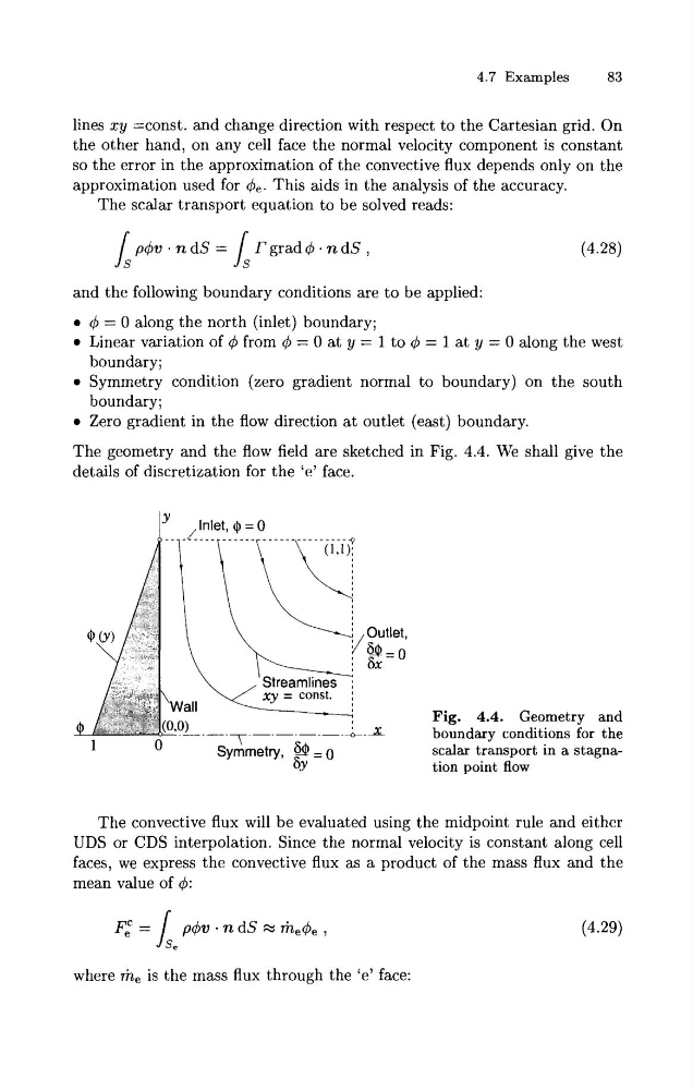
and the following boundary conditions are to be applied:
q5 = 0 along the north (inlet) boundary;
Linear variation of q5 from q5 = 0 a t y = 1 to q5 = 1 a t y = 0 along the west
boundary;
Symmetry condition (zero gradient normal to boundary) on the south
boundary;
Zero gradient in the flow direction a t outlet (east) boundary.
The geometry and the flow field are sketched in Fig. 4.4. We shall give the
details of discretization for the 'e' face.
Fig. 4.4. Geometry and
boundary conditions for the
scalar transport in a stagnation point flow
The convective flux will be evaluated using the midpoint rule and either
UDS or CDS interpolation. Since the normal velocity is constant along cell
faces, we express the convective flux as a product of the mass flux and the
mean value of q5:
where I. is the mass flux through the 'e' face:
83
lines xy =const. and change direction with respect to the Cartesian grid. On
the other hand, on any cell face the normal velocity component is constant
so the error in the approximation of the convective flux depends only on the
approximation used for 4,. This aids in the analysis of the accuracy.
The scalar transport equation to be solved reads:
and the following boundary conditions are to be applied:
q5 = 0 along the north (inlet) boundary;
Linear variation of q5 from q5 = 0 a t y = 1 to q5 = 1 a t y = 0 along the west
boundary;
Symmetry condition (zero gradient normal to boundary) on the south
boundary;
Zero gradient in the flow direction a t outlet (east) boundary.
The geometry and the flow field are sketched in Fig. 4.4. We shall give the
details of discretization for the 'e' face.
Fig. 4.4. Geometry and
boundary conditions for the
scalar transport in a stagnation point flow
The convective flux will be evaluated using the midpoint rule and either
UDS or CDS interpolation. Since the normal velocity is constant along cell
faces, we express the convective flux as a product of the mass flux and the
mean value of q5:
where I. is the mass flux through the 'e' face: