

3.8 The Algebraic Equation System
55
41 =
1842 - 943 + 244 6 Ax 84
11
- -ii- (a,),
Approximations of lower or higher order can be obtained in a similar way.
3.8 The Algebraic Equation System
A finite-difference approximation provides an algebraic equation a t each grid
node; it contains the variable value at that node as well as values at neighboring nodes. If the differential equation is non-linear, the approximation
will contain some non-linear terms. The numerical solution process will then
require linearization; methods for solving these equations will be discussed in
Chap. 5. For now, we consider only the linear case. The methods described
are applicable in the non-linear case as well. For this case, the result of discretization is a system of linear algebraic equations of the form:
where P denotes the node a t which the partial differential equation is approximated and index 1 runs over the neighbor nodes involved in finite-difference
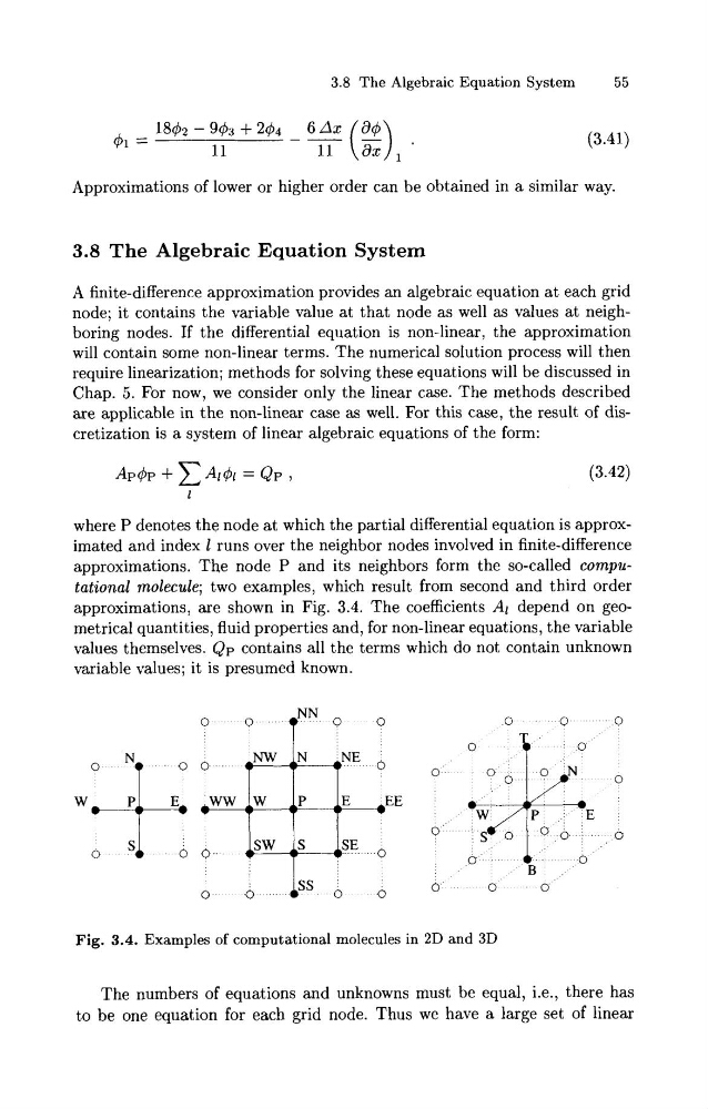
approximations. The node P and its neighbors form the so-called computational molecule; two examples, which result from second and third order
approximations, are shown in Fig. 3.4. The coefficients Al depend on geometrical quantities, fluid properties and, for non-linear equations, the variable
values themselves. Q p contains all the terms which do not contain unknown
variable values; it is presumed known.
Fig. 3.4. Examples of computational molecules in 2D and 3D
The numbers of equations and unknowns must be equal, i.e., there has
to be one equation for each grid node. Thus we have a large set of linear
55
41 =
1842 - 943 + 244 6 Ax 84
11
- -ii- (a,),
Approximations of lower or higher order can be obtained in a similar way.
3.8 The Algebraic Equation System
A finite-difference approximation provides an algebraic equation a t each grid
node; it contains the variable value at that node as well as values at neighboring nodes. If the differential equation is non-linear, the approximation
will contain some non-linear terms. The numerical solution process will then
require linearization; methods for solving these equations will be discussed in
Chap. 5. For now, we consider only the linear case. The methods described
are applicable in the non-linear case as well. For this case, the result of discretization is a system of linear algebraic equations of the form:
where P denotes the node a t which the partial differential equation is approximated and index 1 runs over the neighbor nodes involved in finite-difference
approximations. The node P and its neighbors form the so-called computational molecule; two examples, which result from second and third order
approximations, are shown in Fig. 3.4. The coefficients Al depend on geometrical quantities, fluid properties and, for non-linear equations, the variable
values themselves. Q p contains all the terms which do not contain unknown
variable values; it is presumed known.
Fig. 3.4. Examples of computational molecules in 2D and 3D
The numbers of equations and unknowns must be equal, i.e., there has
to be one equation for each grid node. Thus we have a large set of linear