

3.2 Basic Concept
41
involve derivatives (as in Neumann conditions), the boundary condition must
be discretized to contribute an equation t o the set that must be solved.
The idea behind finite difference approximations is borrowed directly from
the definition of a derivative:
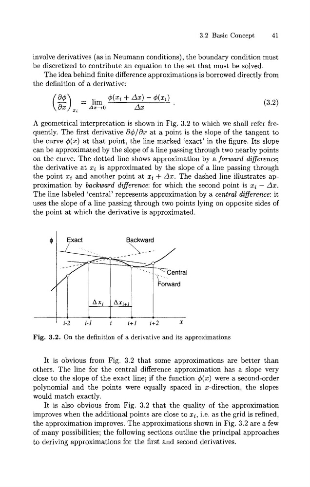
A geometrical interpretation is shown in Fig. 3.2 to which we shall refer frequently. The first derivative aqh/ax at a point is the slope of the tangent to
the curve 4(x) a t that point, the line marked 'exact' in the figure. Its slope
can be approximated by the slope of a line passing through two nearby points
on the curve. The dotted line shows approximation by a forward difference;
the derivative a t xi is approximated by the slope of a line passing through
the point xi and another point at xi + Ax. The dashed line illustrates approximation by backward difference: for which the second point is xi - Ax.
The line labeled 'central' represents approximation by a central difference: it
uses the slope of a line passing through two points lying on opposite sides of
the point at which the derivative is approximated.
Exact
1
B\ackward
Fig. 3.2. On the definition of a derivative and its approximations
Forward
It is obvious from Fig. 3.2 that some approximations are better than
others. The line for the central difference approximation has a slope very
close to the slope of the exact line; if the function 4(x) were a second-order
polynomial and the points were equally spaced in x-direction, the slopes
would match exactly.
It is also obvious from Fig. 3.2 that the quality of the approximation
improves when the additional points are close to xi, i.e. as the grid is refined,
the approximation improves. The approximations shown in Fig. 3.2 are a few
of many possibilities; the following sections outline the principal approaches
to deriving approximations for the first and second derivatives.
1
i-2
i-1
i
i+l
i+2
x
A x i
Axi+,
41
involve derivatives (as in Neumann conditions), the boundary condition must
be discretized to contribute an equation t o the set that must be solved.
The idea behind finite difference approximations is borrowed directly from
the definition of a derivative:
A geometrical interpretation is shown in Fig. 3.2 to which we shall refer frequently. The first derivative aqh/ax at a point is the slope of the tangent to
the curve 4(x) a t that point, the line marked 'exact' in the figure. Its slope
can be approximated by the slope of a line passing through two nearby points
on the curve. The dotted line shows approximation by a forward difference;
the derivative a t xi is approximated by the slope of a line passing through
the point xi and another point at xi + Ax. The dashed line illustrates approximation by backward difference: for which the second point is xi - Ax.
The line labeled 'central' represents approximation by a central difference: it
uses the slope of a line passing through two points lying on opposite sides of
the point at which the derivative is approximated.
Exact
1
B\ackward
Fig. 3.2. On the definition of a derivative and its approximations
Forward
It is obvious from Fig. 3.2 that some approximations are better than
others. The line for the central difference approximation has a slope very
close to the slope of the exact line; if the function 4(x) were a second-order
polynomial and the points were equally spaced in x-direction, the slopes
would match exactly.
It is also obvious from Fig. 3.2 that the quality of the approximation
improves when the additional points are close to xi, i.e. as the grid is refined,
the approximation improves. The approximations shown in Fig. 3.2 are a few
of many possibilities; the following sections outline the principal approaches
to deriving approximations for the first and second derivatives.
1
i-2
i-1
i
i+l
i+2
x
A x i
Axi+,