

11.1 Error Analysis and Estimation
335
uniform grid, which was finer near walls, are an order of magnitude more
accurate than those obtained on a uniform grid with the same number of
nodes. Both solutions converge to the same grid-independent solution with
the same order (second), but the errors differ in magnitude by a factor of 10
or more! Other examples with similar conclusions were shown in Figs. 6.3,
6.5, and 7.18.
The above example stresses the importance of good grid design. For practical engineering applications, grid generation is the most time-consuming
task; it is often difficult to generate any grid, let alone a grid of high quality.
A good grid should be as nearly orthogonal as possible (note that orthogonality has a different meaning in different methods; in a FV method, the
angle between the cell-face normal and the line connecting neighboring cell
centers is what counts - a tetrahedral grid may be orthogonal in this sense).
It should be dense where large truncation errors are expected - hence the
grid designer should know something about the solution. This is the most
important criterion and is best met by using an unstructured grid with local refinement. Other criteria of quality depend on the method used (grid
smoothness, aspect and expansion ratios etc.).
The simplest means of estimation of discretization errors is based on
Richardson extrapolation and assumes that calculations can be done on grids
sufficiently fine that monotone convergence is obtained. (If this is not the case,
it is likely that the error is larger than one would like.) The method is therefore only accurate when the two finest grids are fine enough and the order
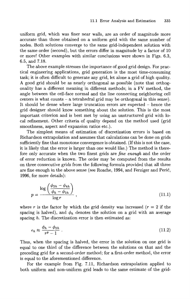
of error reduction is known. The order may be computed from the results
on three consecutive grids from the following formula provided that all three
are fine enough in the above sense (see Roache, 1994, and Ferziger and PeriC,
1996, for more details):
where T is the factor by which the grid density was increased (T = 2 if the
spacing is halved), and Oh denotes the solution on a grid with an average
spacing h. The discretization error is then estimated as:
Thus, when the spacing is halved, the error in the solution on one grid is
equal to one third of the difference between the solutions on that and the
preceding grid for a second-order method; for a first-order method, the error
is equal to the aforementioned difference.
For the example from Fig. 7.11, Richardson extrapolation applied to
both uniform and non-uniform grid leads to the same estimate of the grid-
335
uniform grid, which was finer near walls, are an order of magnitude more
accurate than those obtained on a uniform grid with the same number of
nodes. Both solutions converge to the same grid-independent solution with
the same order (second), but the errors differ in magnitude by a factor of 10
or more! Other examples with similar conclusions were shown in Figs. 6.3,
6.5, and 7.18.
The above example stresses the importance of good grid design. For practical engineering applications, grid generation is the most time-consuming
task; it is often difficult to generate any grid, let alone a grid of high quality.
A good grid should be as nearly orthogonal as possible (note that orthogonality has a different meaning in different methods; in a FV method, the
angle between the cell-face normal and the line connecting neighboring cell
centers is what counts - a tetrahedral grid may be orthogonal in this sense).
It should be dense where large truncation errors are expected - hence the
grid designer should know something about the solution. This is the most
important criterion and is best met by using an unstructured grid with local refinement. Other criteria of quality depend on the method used (grid
smoothness, aspect and expansion ratios etc.).
The simplest means of estimation of discretization errors is based on
Richardson extrapolation and assumes that calculations can be done on grids
sufficiently fine that monotone convergence is obtained. (If this is not the case,
it is likely that the error is larger than one would like.) The method is therefore only accurate when the two finest grids are fine enough and the order
of error reduction is known. The order may be computed from the results
on three consecutive grids from the following formula provided that all three
are fine enough in the above sense (see Roache, 1994, and Ferziger and PeriC,
1996, for more details):
where T is the factor by which the grid density was increased (T = 2 if the
spacing is halved), and Oh denotes the solution on a grid with an average
spacing h. The discretization error is then estimated as:
Thus, when the spacing is halved, the error in the solution on one grid is
equal to one third of the difference between the solutions on that and the
preceding grid for a second-order method; for a first-order method, the error
is equal to the aforementioned difference.
For the example from Fig. 7.11, Richardson extrapolation applied to
both uniform and non-uniform grid leads to the same estimate of the grid-