

10.2 Pressure-Correction Methods for Arbitrary Mach Number
317
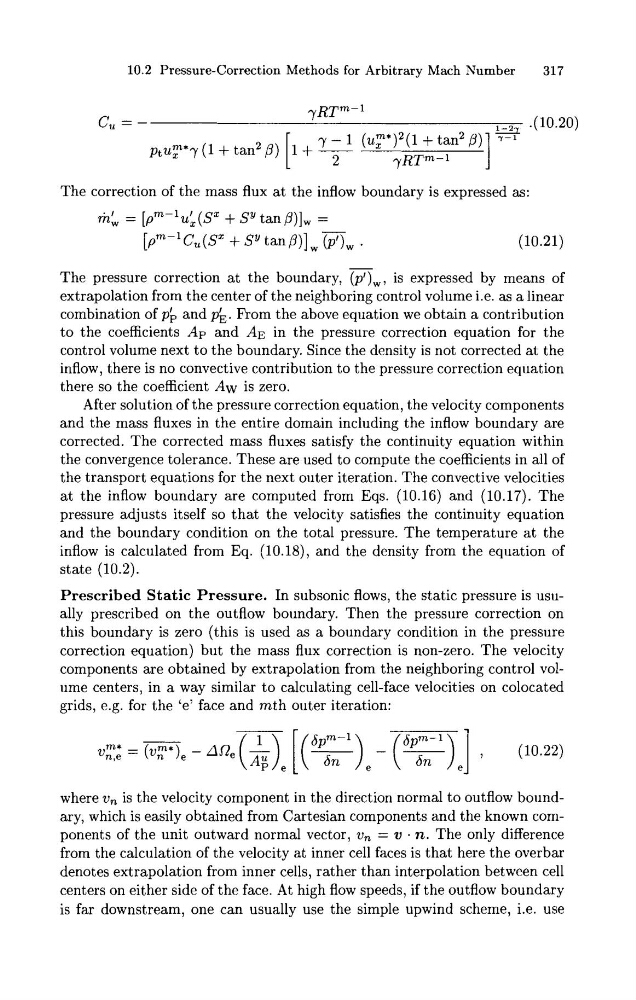
The correction of the mass flux a t the inflow boundary is expressed as:
mk = [pm-l~I,(Sx + SY tanp)], =
[pm-lCu(SZ + SY tanp)],(p'), .
(10.21)
The pressure correction a t the boundary, (p' ),, is expressed by means of
extrapolation from the center of the neighboring control volume i.e. as a linear
combination of pf, and pb. From the above equation we obtain a contribution
to the coefficients Ap and AE in the pressure correction equation for the
control volume next t o the boundary. Since the density is not corrected at the
inflow, there is no convective contribution to the pressure correction equation
there so the coefficient Aw is zero.
After solution of the pressure correction equation, the velocity components
and the mass fluxes in the entire domain including the inflow boundary are
corrected. The corrected mass fluxes satisfy the continuity equation within
the convergence tolerance. These are used to compute the coefficients in all of
the transport equations for the next outer iteration. The convective velocities
a t the inflow boundary are computed from Eqs. (10.16) and (10.17). The
pressure adjusts itself so that the velocity satisfies the continuity equation
and the boundary condition on the total pressure. The temperature a t the
inflow is calculated from Eq. (10.18), and the density from the equation of
state (10.2).
Prescribed Static Pressure. In subsonic flows, the static pressure is usually prescribed on the outflow boundary. Then the pressure correction on
this boundary is zero (this is used as a boundary condition in the pressure
correction equation) but the mass flux correction is non-zero. The velocity
components are obtained by extrapolation from the neighboring control volume centers, in a way similar t o calculating cell-face velocities on colocated
grids, e.g. for the 'e' face and mth outer iteration:
where v, is the velocity component in the direction normal t o outflow boundary, which is easily obtained from Cartesian components and the known components of the unit outward normal vector, v, = v . n. The only difference
from the calculation of the velocity at inner cell faces is that here the overbar
denotes extrapolation from inner cells, rather than interpolation between cell
centers on either side of the face. At high flow speeds, if the outflow boundary
is far downstream, one can usually use the simple upwind scheme, i.e. use
317
The correction of the mass flux a t the inflow boundary is expressed as:
mk = [pm-l~I,(Sx + SY tanp)], =
[pm-lCu(SZ + SY tanp)],(p'), .
(10.21)
The pressure correction a t the boundary, (p' ),, is expressed by means of
extrapolation from the center of the neighboring control volume i.e. as a linear
combination of pf, and pb. From the above equation we obtain a contribution
to the coefficients Ap and AE in the pressure correction equation for the
control volume next t o the boundary. Since the density is not corrected at the
inflow, there is no convective contribution to the pressure correction equation
there so the coefficient Aw is zero.
After solution of the pressure correction equation, the velocity components
and the mass fluxes in the entire domain including the inflow boundary are
corrected. The corrected mass fluxes satisfy the continuity equation within
the convergence tolerance. These are used to compute the coefficients in all of
the transport equations for the next outer iteration. The convective velocities
a t the inflow boundary are computed from Eqs. (10.16) and (10.17). The
pressure adjusts itself so that the velocity satisfies the continuity equation
and the boundary condition on the total pressure. The temperature a t the
inflow is calculated from Eq. (10.18), and the density from the equation of
state (10.2).
Prescribed Static Pressure. In subsonic flows, the static pressure is usually prescribed on the outflow boundary. Then the pressure correction on
this boundary is zero (this is used as a boundary condition in the pressure
correction equation) but the mass flux correction is non-zero. The velocity
components are obtained by extrapolation from the neighboring control volume centers, in a way similar t o calculating cell-face velocities on colocated
grids, e.g. for the 'e' face and mth outer iteration:
where v, is the velocity component in the direction normal t o outflow boundary, which is easily obtained from Cartesian components and the known components of the unit outward normal vector, v, = v . n. The only difference
from the calculation of the velocity at inner cell faces is that here the overbar
denotes extrapolation from inner cells, rather than interpolation between cell
centers on either side of the face. At high flow speeds, if the outflow boundary
is far downstream, one can usually use the simple upwind scheme, i.e. use