

8.11 Examples
259
mass flow rate is not known, but the pressures at the inlet and outlet are
prescribed. Also, pressure is sometimes specified at a far field boundary.
When the pressure is specified at a boundary, velocity cannot be prescribed - it has t o be extrapolated from the interior using the same approach
as for cell faces between two CVs, see Eq. (8.51). The pressure gradient at
the boundary is approximated using one-sided differences; for example, at
the 'e' face, one can use expression (8.26), which is a first order backward
difference.
The boundary velocities determined in this way need to be corrected to
satisfy the mass conservation; the mass flux corrections m' are not zero a t
boundaries where the pressure is specified. However, boundary pressure is
not corrected, i.e. p' = 0 a t boundary. This is used as a Dirichlet boundary
condition in the pressure-correction equation.
If the Reynolds number is high, the solution process will converge slowly
if the above approach is applied when the inlet and outlet pressures are
specified. Another possibility is to guess first the mass flow rate at inlet and
treat it as prescribed for one outer iteration, and consider the pressure to be
specified only a t outlet. The inlet velocities should then be corrected by trying
to match the extrapolated pressure at the inlet boundary with the specified
pressure. An iterative correction procedure is used to drive the difference
between two pressures to zero.
8.11 Examples
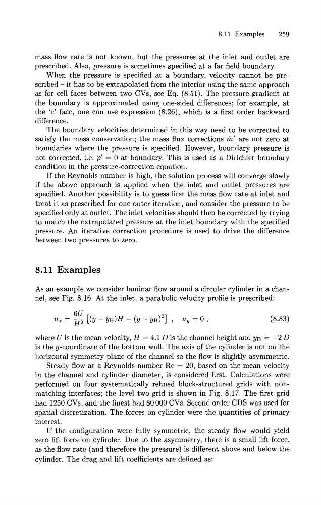
As an example we consider laminar flow around a circular cylinder in a channel, see Fig. 8.16. At the inlet, a parabolic velocity profile is prescribed:
where U is the mean velocity, H = 4.1 D is the channel height and y~ = -2 D
is the y-coordinate of the bottom wall. The axis of the cylinder is not on the
horizontal symmetry plane of the channel so the flow is slightly asymmetric.
Steady flow a t a Reynolds number Re = 20, based on the mean velocity
in the channel and cylinder diameter, is considered first. Calculations were
performed on four systematically refined block-structured grids with nonmatching interfaces; the level two grid is shown in Fig. 8.17. The first grid
had 1250 CVs, and the finest had 80 000 CVs. Second order CDS was used for
spatial discretization. The forces on cylinder were the quantities of primary
interest.
If the configuration were fully symmetric, the steady flow would yield
zero lift force on cylinder. Due to the asymmetry, there is a small lift force,
as the flow rate (and therefore the pressure) is different above and below the
cylinder. The drag and lift coefficients are defined as:
259
mass flow rate is not known, but the pressures at the inlet and outlet are
prescribed. Also, pressure is sometimes specified at a far field boundary.
When the pressure is specified at a boundary, velocity cannot be prescribed - it has t o be extrapolated from the interior using the same approach
as for cell faces between two CVs, see Eq. (8.51). The pressure gradient at
the boundary is approximated using one-sided differences; for example, at
the 'e' face, one can use expression (8.26), which is a first order backward
difference.
The boundary velocities determined in this way need to be corrected to
satisfy the mass conservation; the mass flux corrections m' are not zero a t
boundaries where the pressure is specified. However, boundary pressure is
not corrected, i.e. p' = 0 a t boundary. This is used as a Dirichlet boundary
condition in the pressure-correction equation.
If the Reynolds number is high, the solution process will converge slowly
if the above approach is applied when the inlet and outlet pressures are
specified. Another possibility is to guess first the mass flow rate at inlet and
treat it as prescribed for one outer iteration, and consider the pressure to be
specified only a t outlet. The inlet velocities should then be corrected by trying
to match the extrapolated pressure at the inlet boundary with the specified
pressure. An iterative correction procedure is used to drive the difference
between two pressures to zero.
8.11 Examples
As an example we consider laminar flow around a circular cylinder in a channel, see Fig. 8.16. At the inlet, a parabolic velocity profile is prescribed:
where U is the mean velocity, H = 4.1 D is the channel height and y~ = -2 D
is the y-coordinate of the bottom wall. The axis of the cylinder is not on the
horizontal symmetry plane of the channel so the flow is slightly asymmetric.
Steady flow a t a Reynolds number Re = 20, based on the mean velocity
in the channel and cylinder diameter, is considered first. Calculations were
performed on four systematically refined block-structured grids with nonmatching interfaces; the level two grid is shown in Fig. 8.17. The first grid
had 1250 CVs, and the finest had 80 000 CVs. Second order CDS was used for
spatial discretization. The forces on cylinder were the quantities of primary
interest.
If the configuration were fully symmetric, the steady flow would yield
zero lift force on cylinder. Due to the asymmetry, there is a small lift force,
as the flow rate (and therefore the pressure) is different above and below the
cylinder. The drag and lift coefficients are defined as: