

242
8. Complex Geometries
where O3 is the offset for block 3 (the number of nodes in all preceding blocks,
i.e. N,!N,! + N,"N,j' ) and N, " and Njm are the numbers of nodes in the i and
j directions in block m.
mn
Block B
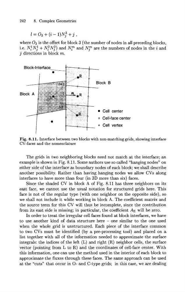
Fig. 8.11. Interface between two blocks with non-matching grids, showing interface
CV-faces and the nomenclature
The grids in two neighboring blocks need not match at the interface; an
example is shown in Fig. 8.11. Some authors use so called "hanging nodes" on
either side of the interface as boundary nodes of each block; we shall describe
another possibility. Rather than having hanging nodes we allow CVs along
interfaces to have more than four (in 3D more than six) faces.
Since the shaded CV in block A of Fig. 8.11 has three neighbors on its
east face, we cannot use the usual notation for structured grids here. This
face is not of the regular type (with one neighbor on the opposite side), so
we shall not include it while working in block A. The coefficient matrix and
the source term for this CV will thus be incomplete, since the contribution
from its east side is missing; in particular, the coefficient AE will be zero.
In order to treat the irregular cell faces found at block interfaces, we have
to use another kind of data structure here - one similar to the one used
when the whole grid is unstructured. Each piece of the interface common
to two CVs must be identified (by a pre-processing tool) and placed on a
list together with all of the information needed to approximate the surface
integrals: the indices of the left (L) and right (R) neighbor cells, the surface
vector (pointing from L to R) and the coordinates of cell-face center. With
this information, one can use the method used in the interior of each block to
approximate the fluxes through these faces. The same approach can be used
at the "cuts" that occur in 0- and C-type grids; in this case, we are dealing
8. Complex Geometries
where O3 is the offset for block 3 (the number of nodes in all preceding blocks,
i.e. N,!N,! + N,"N,j' ) and N, " and Njm are the numbers of nodes in the i and
j directions in block m.
mn
Block B
Fig. 8.11. Interface between two blocks with non-matching grids, showing interface
CV-faces and the nomenclature
The grids in two neighboring blocks need not match at the interface; an
example is shown in Fig. 8.11. Some authors use so called "hanging nodes" on
either side of the interface as boundary nodes of each block; we shall describe
another possibility. Rather than having hanging nodes we allow CVs along
interfaces to have more than four (in 3D more than six) faces.
Since the shaded CV in block A of Fig. 8.11 has three neighbors on its
east face, we cannot use the usual notation for structured grids here. This
face is not of the regular type (with one neighbor on the opposite side), so
we shall not include it while working in block A. The coefficient matrix and
the source term for this CV will thus be incomplete, since the contribution
from its east side is missing; in particular, the coefficient AE will be zero.
In order to treat the irregular cell faces found at block interfaces, we have
to use another kind of data structure here - one similar to the one used
when the whole grid is unstructured. Each piece of the interface common
to two CVs must be identified (by a pre-processing tool) and placed on a
list together with all of the information needed to approximate the surface
integrals: the indices of the left (L) and right (R) neighbor cells, the surface
vector (pointing from L to R) and the coordinates of cell-face center. With
this information, one can use the method used in the interior of each block to
approximate the fluxes through these faces. The same approach can be used
at the "cuts" that occur in 0- and C-type grids; in this case, we are dealing