

228
8. Complex Geometries
in the diffusive terms. In order to show this clearly, we rewrite the Eq. (8.5)
in the expanded form:
All three derivatives of 4, which stem from the gradient operator, appear
inside each of the outer derivatives, which stem from the divergence operator,
see Eq. (1.27). The mixed derivatives of 4 are multiplied by coefficients Bmj
with unequal indices, which become zero when the grid is orthogonal, whether
it is rectilinear or curvilinear. If the grid is non-orthogonal, their magnitudes
relative to the diagonal elements Bii depend on the angles between the grid
lines and on the grid aspect ratio. When the angle between grid lines is
small and the aspect ratio large, the coefficients multiplying mixed derivatives
may be larger than the diagonal coefficients, which can lead to numerical
problems (poor convergence, oscillations in the solution etc.). If the nonorthogonality and aspect ratio are moderate, these terms are much smaller
than the diagonal ones and cause no problems. The mixed derivative terms
are usually treated explicitly, as their inclusion in the implicit computational
molecule would make the latter large and solution more expensive. Explicit
treatment usually increases the number of outer iterations, but the savings
derived from simpler and less expensive inner iterations is far more significant.
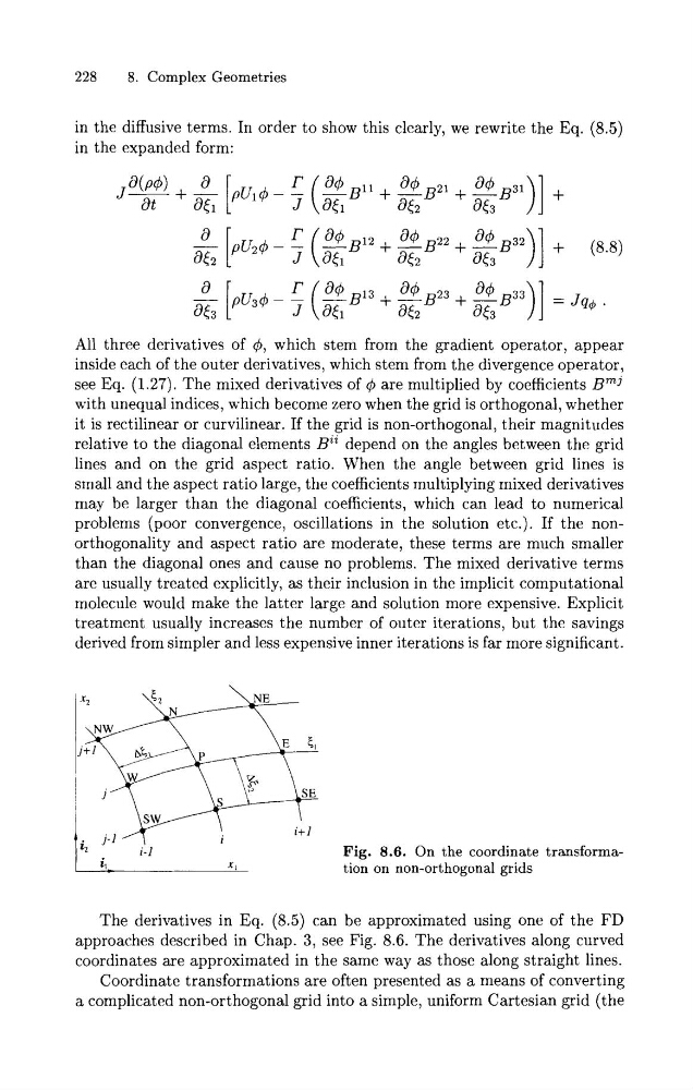
Fig. 8.6. On the coordinate transformation on non-orthogonal grids
The derivatives in Eq. (8.5) can be approximated using one of the FD
approaches described in Chap. 3, see Fig. 8.6. The derivatives along curved
coordinates are approximated in the same way as those along straight lines.
Coordinate transformations are often presented as a means of converting
a complicated non-orthogonal grid into a simple, uniform Cartesian grid (the
8. Complex Geometries
in the diffusive terms. In order to show this clearly, we rewrite the Eq. (8.5)
in the expanded form:
All three derivatives of 4, which stem from the gradient operator, appear
inside each of the outer derivatives, which stem from the divergence operator,
see Eq. (1.27). The mixed derivatives of 4 are multiplied by coefficients Bmj
with unequal indices, which become zero when the grid is orthogonal, whether
it is rectilinear or curvilinear. If the grid is non-orthogonal, their magnitudes
relative to the diagonal elements Bii depend on the angles between the grid
lines and on the grid aspect ratio. When the angle between grid lines is
small and the aspect ratio large, the coefficients multiplying mixed derivatives
may be larger than the diagonal coefficients, which can lead to numerical
problems (poor convergence, oscillations in the solution etc.). If the nonorthogonality and aspect ratio are moderate, these terms are much smaller
than the diagonal ones and cause no problems. The mixed derivative terms
are usually treated explicitly, as their inclusion in the implicit computational
molecule would make the latter large and solution more expensive. Explicit
treatment usually increases the number of outer iterations, but the savings
derived from simpler and less expensive inner iterations is far more significant.
Fig. 8.6. On the coordinate transformation on non-orthogonal grids
The derivatives in Eq. (8.5) can be approximated using one of the FD
approaches described in Chap. 3, see Fig. 8.6. The derivatives along curved
coordinates are approximated in the same way as those along straight lines.
Coordinate transformations are often presented as a means of converting
a complicated non-orthogonal grid into a simple, uniform Cartesian grid (the