

226
8. Complex Geometries
components are stored at each CV face. However, this becomes complicated
in 3D, especially if CVs of arbitrary shape are allowed. To see how this may
be done, interested readers may want to look at the paper by Maliska and
Raithby (1984).
--, Velocities
0 Pressure
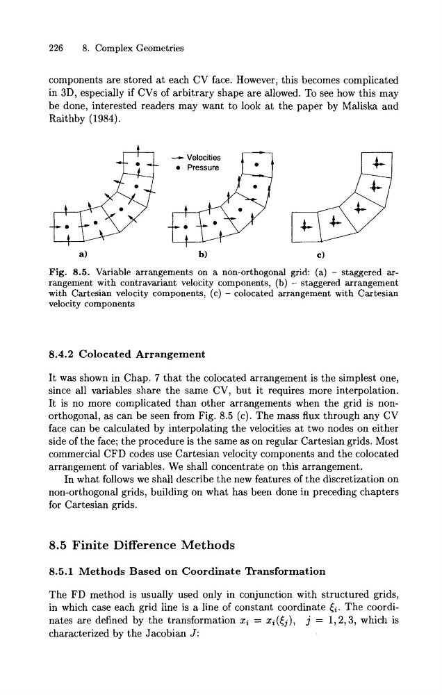
Fig. 8.5. Variable arrangements on a non-orthogonal grid: (a) - staggered arrangement with contravariant velocity components, (b) - staggered arrangement
with Cartesian velocity components, (c) - colocated arrangement with Cartesian
velocity components
8.4.2 Colocated Arrangement
It was shown in Chap. 7 that the colocated arrangement is the simplest one,
since all variables share the same CV, but it requires more interpolation.
It is no more complicated than other arrangements when the grid is nonorthogonal, as can be seen from Fig. 8.5 (c). The mass flux through any CV
face can be calculated by interpolating the velocities at two nodes on either
side of the face; the procedure is the same as on regular Cartesian grids. Most
commercial CFD codes use Cartesian velocity components and the colocated
arrangement of variables. We shall concentrate on this arrangement.
In what follows we shall describe the new features of the discretization on
non-orthogonal grids, building on what has been done in preceding chapters
for Cartesian grids.
8.5 Finite Difference Methods
8.5.1 Methods Based on Coordinate Transformation
The FD method is usually used only in conjunction with structured grids,
in which case each grid line is a line of constant coordinate &. The coordinates are defined by the transformation xi = xi ( J j ) , j = 1,2,3, which is
characterized by the Jacobian J:
8. Complex Geometries
components are stored at each CV face. However, this becomes complicated
in 3D, especially if CVs of arbitrary shape are allowed. To see how this may
be done, interested readers may want to look at the paper by Maliska and
Raithby (1984).
--, Velocities
0 Pressure
Fig. 8.5. Variable arrangements on a non-orthogonal grid: (a) - staggered arrangement with contravariant velocity components, (b) - staggered arrangement
with Cartesian velocity components, (c) - colocated arrangement with Cartesian
velocity components
8.4.2 Colocated Arrangement
It was shown in Chap. 7 that the colocated arrangement is the simplest one,
since all variables share the same CV, but it requires more interpolation.
It is no more complicated than other arrangements when the grid is nonorthogonal, as can be seen from Fig. 8.5 (c). The mass flux through any CV
face can be calculated by interpolating the velocities at two nodes on either
side of the face; the procedure is the same as on regular Cartesian grids. Most
commercial CFD codes use Cartesian velocity components and the colocated
arrangement of variables. We shall concentrate on this arrangement.
In what follows we shall describe the new features of the discretization on
non-orthogonal grids, building on what has been done in preceding chapters
for Cartesian grids.
8.5 Finite Difference Methods
8.5.1 Methods Based on Coordinate Transformation
The FD method is usually used only in conjunction with structured grids,
in which case each grid line is a line of constant coordinate &. The coordinates are defined by the transformation xi = xi ( J j ) , j = 1,2,3, which is
characterized by the Jacobian J: