

7.3 Calculation of the Pressure
173
Many solution methods for steady incompressible flows are of the latter
type; some of the most popular ones can be regarded as variations on the
method of the preceding section. They use a pressure (or pressure-correction)
equation to enforce mass conservation at each time step or, in the language
preferred for steady solvers, each outer iteration. We now look at some of
these methods.
If an implicit method is used to advance the momentum equations in
time, the discretized equations for the velocities a t the new time step are
non-linear. If the pressure gradient term is not included in the source term,
these may be written:
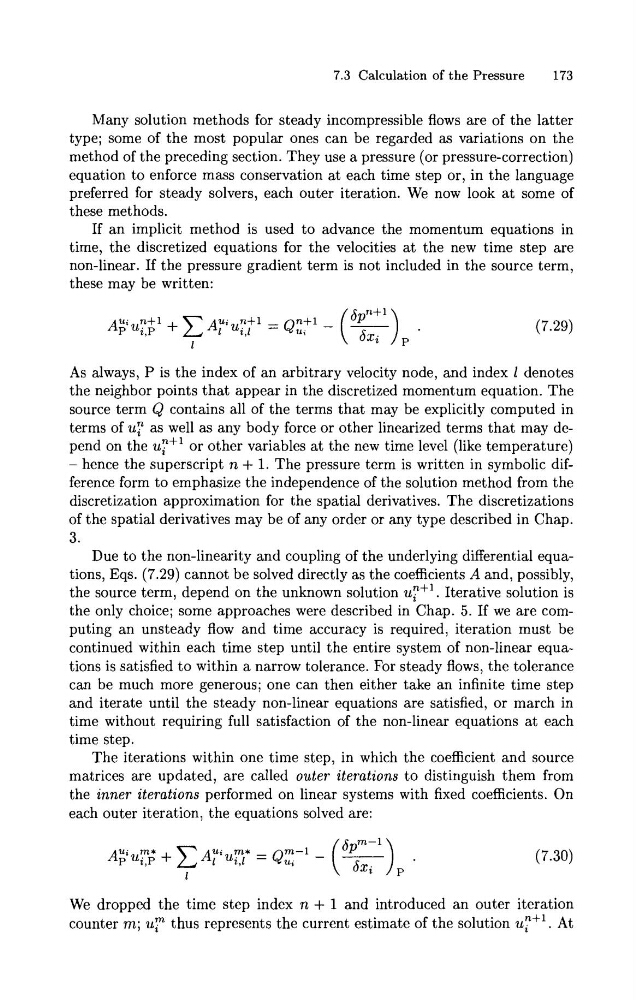
As always, P is the index of an arbitrary velocity node, and index 1 denotes
the neighbor points that appear in the discretized momentum equation. The
source term Q contains all of the terms that may be explicitly computed in
terms of ur as well as any body force or other linearized terms that may depend on the u : + ' or other variables a t the new time level (like temperature)
- hence the superscript n + 1. The pressure term is written in symbolic difference form to emphasize the independence of the solution method from the
discretization approximation for the spatial derivatives. The discretizations
of the spatial derivatives may be of any order or any type described in Chap.
3.
Due to the non-linearity and coupling of the underlying differential equations, Eqs. (7.29) cannot be solved directly as the coefficients A and, possibly,
the source term, depend on the unknown solution u:+l. Iterative solution is
the only choice; some approaches were described in Chap. 5. If we are computing an unsteady flow and time accuracy is required, iteration must be
continued within each time step until the entire system of non-linear equations is satisfied t o within a narrow tolerance. For steady flows, the tolerance
can be much more generous; one can then either take an infinite time step
and iterate until the steady non-linear equations are satisfied, or march in
time without requiring full satisfaction of the non-linear equations at each
time step.
The iterations within one time step, in which the coefficient and source
matrices are updated, are called outer iterations t o distinguish them from
the inner iterations performed on linear systems with fixed coefficients. On
each outer iteration, the equations solved are:
We dropped the time step index n + 1 and introduced an outer iteration
counter m; uy thus represents the current estimate of the solution uy+l. At
173
Many solution methods for steady incompressible flows are of the latter
type; some of the most popular ones can be regarded as variations on the
method of the preceding section. They use a pressure (or pressure-correction)
equation to enforce mass conservation at each time step or, in the language
preferred for steady solvers, each outer iteration. We now look at some of
these methods.
If an implicit method is used to advance the momentum equations in
time, the discretized equations for the velocities a t the new time step are
non-linear. If the pressure gradient term is not included in the source term,
these may be written:
As always, P is the index of an arbitrary velocity node, and index 1 denotes
the neighbor points that appear in the discretized momentum equation. The
source term Q contains all of the terms that may be explicitly computed in
terms of ur as well as any body force or other linearized terms that may depend on the u : + ' or other variables a t the new time level (like temperature)
- hence the superscript n + 1. The pressure term is written in symbolic difference form to emphasize the independence of the solution method from the
discretization approximation for the spatial derivatives. The discretizations
of the spatial derivatives may be of any order or any type described in Chap.
3.
Due to the non-linearity and coupling of the underlying differential equations, Eqs. (7.29) cannot be solved directly as the coefficients A and, possibly,
the source term, depend on the unknown solution u:+l. Iterative solution is
the only choice; some approaches were described in Chap. 5. If we are computing an unsteady flow and time accuracy is required, iteration must be
continued within each time step until the entire system of non-linear equations is satisfied t o within a narrow tolerance. For steady flows, the tolerance
can be much more generous; one can then either take an infinite time step
and iterate until the steady non-linear equations are satisfied, or march in
time without requiring full satisfaction of the non-linear equations at each
time step.
The iterations within one time step, in which the coefficient and source
matrices are updated, are called outer iterations t o distinguish them from
the inner iterations performed on linear systems with fixed coefficients. On
each outer iteration, the equations solved are:
We dropped the time step index n + 1 and introduced an outer iteration
counter m; uy thus represents the current estimate of the solution uy+l. At