

6.3 Application to the Generic Transport Equation
143
the discretized right hand side of the above equation is required at the new
time level, for which the solution is not known yet. Therefore, an algebraic
system of equations, which differs from the one obtained for steady problems,
must be solved. We shall analyze properties of some of the common schemes
when applied to a 1D problem below; solutions of a 1D and a 2D problem
will be discussed in the examples section.
6.3.1 Explicit Methods
Explicit Euler Method. The simplest method is explicit Euler in which
all fluxes and sources are evaluated using known values at t,. In the equation
for a CV or grid point, the only unknown at the new time level is the value at
that node; the neighbor values are all evaluated a t earlier time levels. Thus
one can explicitly calculate the new value of the unknown at each node.
In order to study properties of the explicit Euler and other simple schemes,
we consider the 1D version of Eq. (6.22) with constant velocity, constant fluid
properties, and no source terms:
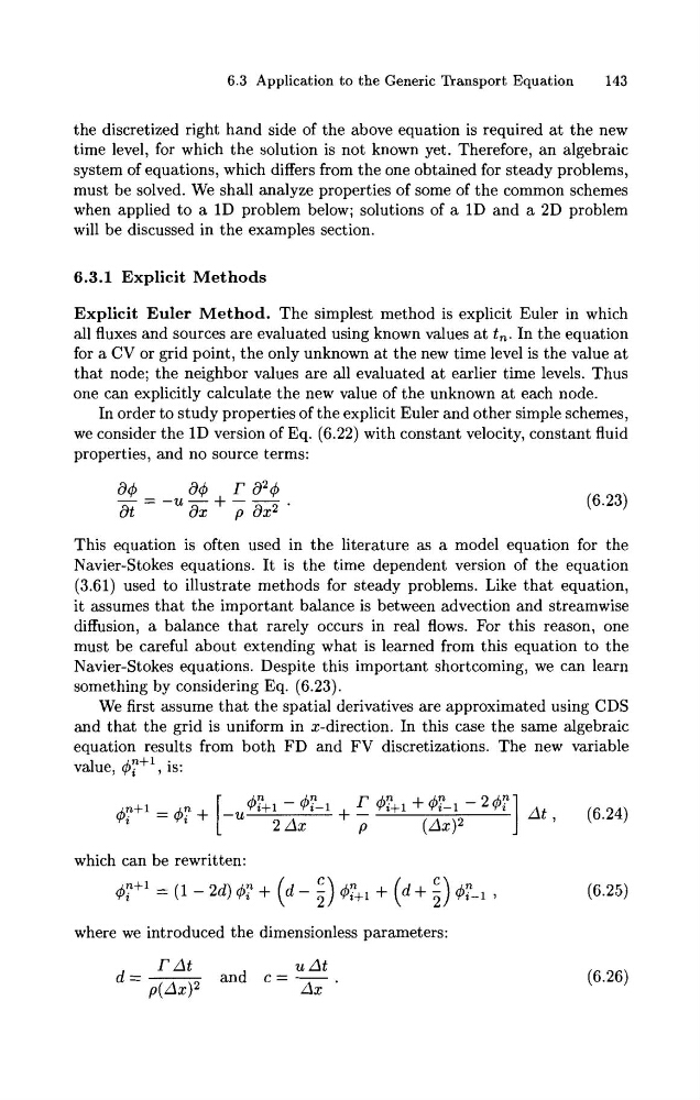
This equation is often used in the literature as a model equation for the
Navier-Stokes equations. It is the time dependent version of the equation
(3.61) used to illustrate methods for steady problems. Like that equation,
it assumes that the important balance is between advection and streamwise
diffusion, a balance that rarely occurs in real flows. For this reason, one
must be careful about extending what is learned from this equation to the
Navier-Stokes equations. Despite this important shortcoming, we can learn
something by considering Eq. (6.23).
We first assume that the spatial derivatives are approximated using CDS
and that the grid is uniform in x-direction. In this case the same algebraic
equation results from both FD and FV discretizations. The new variable
value,
is:
which can be rewritten:
4Yt1 = (1 - 2d) 4; + (d - i) + (d + i) 4:-1 ,
where we introduced the dimensionless parameters:
r At
d = -
u At
and c = -
p ( W 2
Ax
143
the discretized right hand side of the above equation is required at the new
time level, for which the solution is not known yet. Therefore, an algebraic
system of equations, which differs from the one obtained for steady problems,
must be solved. We shall analyze properties of some of the common schemes
when applied to a 1D problem below; solutions of a 1D and a 2D problem
will be discussed in the examples section.
6.3.1 Explicit Methods
Explicit Euler Method. The simplest method is explicit Euler in which
all fluxes and sources are evaluated using known values at t,. In the equation
for a CV or grid point, the only unknown at the new time level is the value at
that node; the neighbor values are all evaluated a t earlier time levels. Thus
one can explicitly calculate the new value of the unknown at each node.
In order to study properties of the explicit Euler and other simple schemes,
we consider the 1D version of Eq. (6.22) with constant velocity, constant fluid
properties, and no source terms:
This equation is often used in the literature as a model equation for the
Navier-Stokes equations. It is the time dependent version of the equation
(3.61) used to illustrate methods for steady problems. Like that equation,
it assumes that the important balance is between advection and streamwise
diffusion, a balance that rarely occurs in real flows. For this reason, one
must be careful about extending what is learned from this equation to the
Navier-Stokes equations. Despite this important shortcoming, we can learn
something by considering Eq. (6.23).
We first assume that the spatial derivatives are approximated using CDS
and that the grid is uniform in x-direction. In this case the same algebraic
equation results from both FD and FV discretizations. The new variable
value,
is:
which can be rewritten:
4Yt1 = (1 - 2d) 4; + (d - i) + (d + i) 4:-1 ,
where we introduced the dimensionless parameters:
r At
d = -
u At
and c = -
p ( W 2
Ax