

136
6. Methods for Unsteady Problems
where we use the shorthand notation Qn+' = 4(tn+'). This equation is exact. However, the right hand side cannot be evaluated without knowing the
solution so some approximation is necessary. The mean value theorem of calculus guarantees that if the integrand is evaluated at the proper point t = T
between tn and tn+', the integral is equal to f (T, Q(T)) At but this is of little use since T is unknown. We therefore use some approximate numerical
quadrature to evaluate the integral.
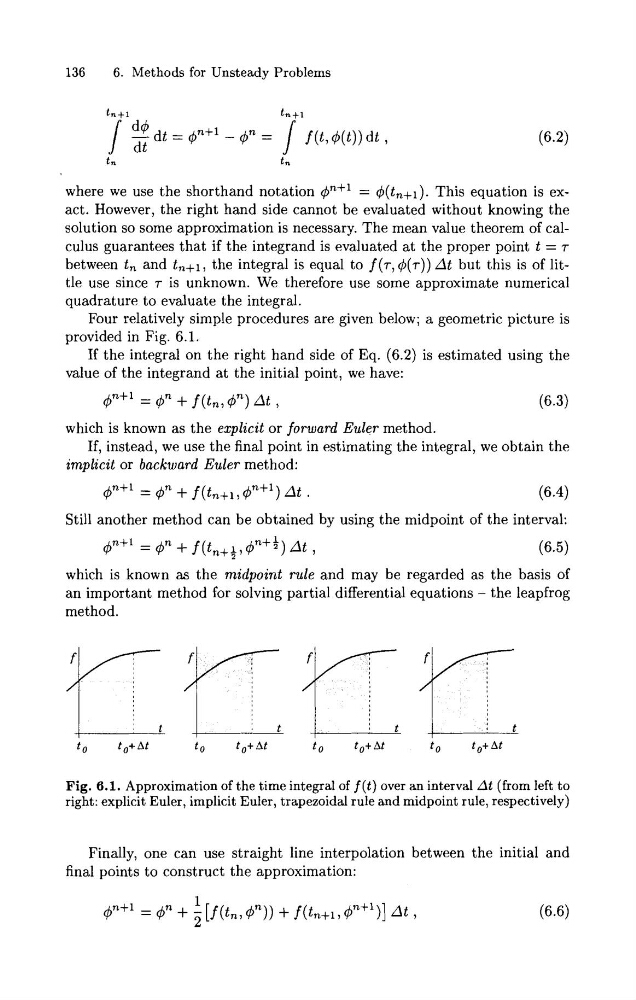
Four relatively simple procedures are given below; a geometric picture is
provided in Fig. 6.1.
If the integral on the right hand side of Eq. (6.2) is estimated using the
value of the integrand at the initial point, we have:
mn+' = 4" + f (tn, Qn) At
(6.3)
which is known as the explicit or forward Euler method.
If, instead, we use the final point in estimating the integral, we obtain the
implicit or backward Euler method:
Still another method can be obtained by using the midpoint of the interval:
mn+l = Qn + f (tn+i,$n+t) A t ,
(6.5)
which is known as the midpoint rule and may be regarded as the basis of
an important method for solving partial differential equations - the leapfrog
method.
Fig. 6.1. Approximation of the time integral of f (t) over an interval At (from left to
right: explicit Euler, implicit Euler, trapezoidal rule and midpoint rule, respectively)
Finally, one can use straight line interpolation between the initial and
final points to construct the approximation:
6. Methods for Unsteady Problems
where we use the shorthand notation Qn+' = 4(tn+'). This equation is exact. However, the right hand side cannot be evaluated without knowing the
solution so some approximation is necessary. The mean value theorem of calculus guarantees that if the integrand is evaluated at the proper point t = T
between tn and tn+', the integral is equal to f (T, Q(T)) At but this is of little use since T is unknown. We therefore use some approximate numerical
quadrature to evaluate the integral.
Four relatively simple procedures are given below; a geometric picture is
provided in Fig. 6.1.
If the integral on the right hand side of Eq. (6.2) is estimated using the
value of the integrand at the initial point, we have:
mn+' = 4" + f (tn, Qn) At
(6.3)
which is known as the explicit or forward Euler method.
If, instead, we use the final point in estimating the integral, we obtain the
implicit or backward Euler method:
Still another method can be obtained by using the midpoint of the interval:
mn+l = Qn + f (tn+i,$n+t) A t ,
(6.5)
which is known as the midpoint rule and may be regarded as the basis of
an important method for solving partial differential equations - the leapfrog
method.
Fig. 6.1. Approximation of the time integral of f (t) over an interval At (from left to
right: explicit Euler, implicit Euler, trapezoidal rule and midpoint rule, respectively)
Finally, one can use straight line interpolation between the initial and
final points to construct the approximation: