

132
5. Solution of Linear Equation Systems
0
50
100
150
200
0
50
100
150
200
Iter.
Iter.
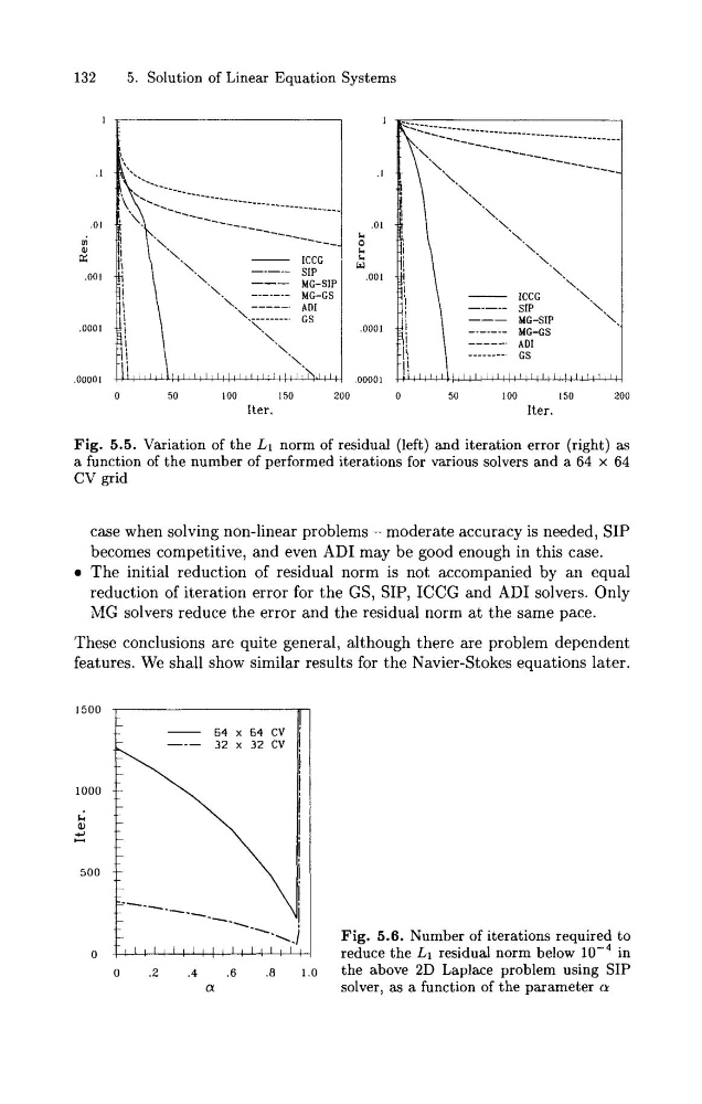
Fig. 5.5. Variation of the L1 norm of residual (left) and iteration error (right) as
a function of the number of performed iterations for various solvers and a 64 x 64
CV grid
case when solving non-linear problems - moderate accuracy is needed, SIP
becomes competitive, and even AD1 may be good enough in this case.
The initial reduction of residual norm is not accompanied by an equal
reduction of iteration error for the GS, SIP, ICCG and AD1 solvers. Only
MG solvers reduce the error and the residual norm a t the same pace.
These conclusions are quite general, although there are problem dependent
features. We shall show similar results for the Navier-Stokes equations later.
- 64 x 64 CV
-
-
/
Fig. 5.6. Number of iterations required to
l l , l ~ l l l l l ~ l l l ~ l ~ l l
7 i
. ,
I , .
reduce the L1 residual norm below
in
o
.2
.4
.6
.a
1.0
the above 2D Laplace problem using SIP
a
solver, as a function of the parameter CI
5. Solution of Linear Equation Systems
0
50
100
150
200
0
50
100
150
200
Iter.
Iter.
Fig. 5.5. Variation of the L1 norm of residual (left) and iteration error (right) as
a function of the number of performed iterations for various solvers and a 64 x 64
CV grid
case when solving non-linear problems - moderate accuracy is needed, SIP
becomes competitive, and even AD1 may be good enough in this case.
The initial reduction of residual norm is not accompanied by an equal
reduction of iteration error for the GS, SIP, ICCG and AD1 solvers. Only
MG solvers reduce the error and the residual norm a t the same pace.
These conclusions are quite general, although there are problem dependent
features. We shall show similar results for the Navier-Stokes equations later.
- 64 x 64 CV
-
-
/
Fig. 5.6. Number of iterations required to
l l , l ~ l l l l l ~ l l l ~ l ~ l l
7 i
. ,
I , .
reduce the L1 residual norm below
in
o
.2
.4
.6
.a
1.0
the above 2D Laplace problem using SIP
a
solver, as a function of the parameter CI