

5.2 Direct Methods
95
5.2.3 Tridiagonal Systems
When ordinary differential equations (ID problems) are finite differenced, for
example, with the CDS approximation, the resulting algebraic equations have
an especially simple structure. Each equation contains only the variables a t
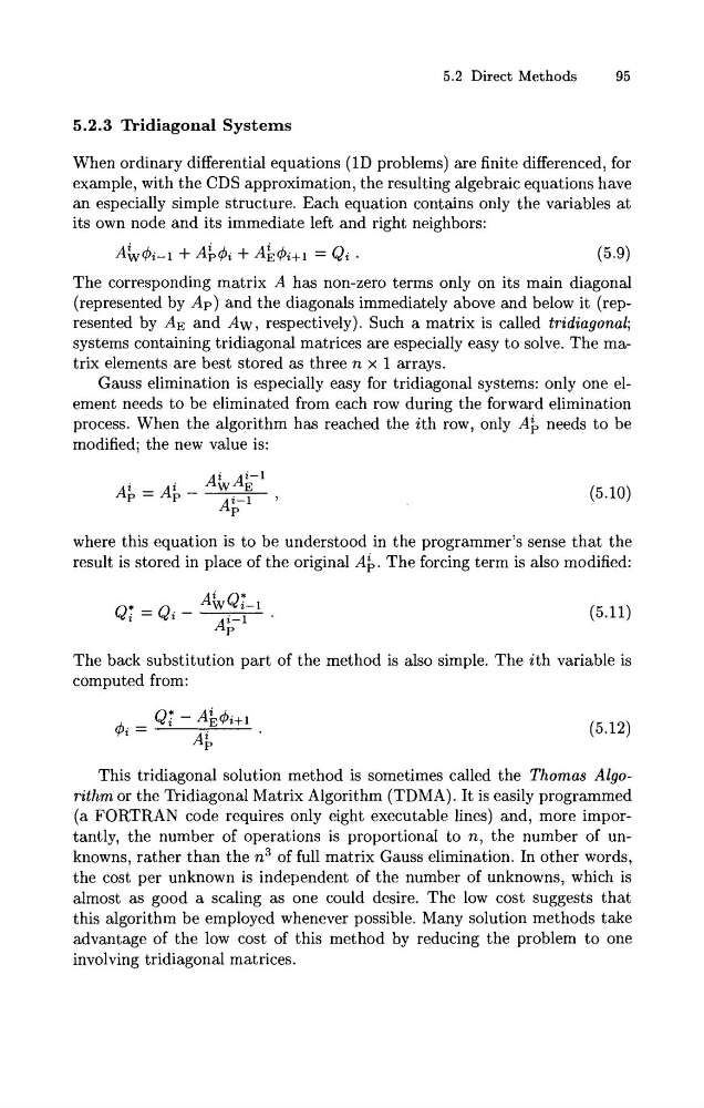
its own node and its immediate left and right neighbors:
The corresponding matrix A has non-zero terms only on its main diagonal
(represented by Ap) and the diagonals immediately above and below it (represented by AE and Aw, respectively). Such a matrix is called tridiagonal;
systems containing tridiagonal matrices are especially easy to solve. The matrix elements are best stored as three n x 1 arrays.
Gauss elimination is especially easy for tridiagonal systems: only one element needs to be eliminated from each row during the forward elimination
process. When the algorithm has reached the ith row, only A$ needs to be
modified; the new value is:
where this equation is to be understood in the programmer's sense that the
result is stored in place of the original A;. The forcing term is also modified:
The back substitution part of the method is also simple. The ith variable is
computed from:
This tridiagonal solution method is sometimes called the Thomas Algorithm or the Tridiagonal Matrix Algorithm (TDMA). It is easily programmed
(a FORTRAN code requires only eight executable lines) and, more importantly, the number of operations is proportional to n , the number of unknowns, rather than the n3 of full matrix Gauss elimination. In other words,
the cost per unknown is independent of the number of unknowns, which is
almost as good a scaling as one could desire. The low cost suggests that
this algorithm be employed whenever possible. Many solution methods take
advantage of the low cost of this method by reducing the problem to one
involving tridiagonal matrices.
95
5.2.3 Tridiagonal Systems
When ordinary differential equations (ID problems) are finite differenced, for
example, with the CDS approximation, the resulting algebraic equations have
an especially simple structure. Each equation contains only the variables a t
its own node and its immediate left and right neighbors:
The corresponding matrix A has non-zero terms only on its main diagonal
(represented by Ap) and the diagonals immediately above and below it (represented by AE and Aw, respectively). Such a matrix is called tridiagonal;
systems containing tridiagonal matrices are especially easy to solve. The matrix elements are best stored as three n x 1 arrays.
Gauss elimination is especially easy for tridiagonal systems: only one element needs to be eliminated from each row during the forward elimination
process. When the algorithm has reached the ith row, only A$ needs to be
modified; the new value is:
where this equation is to be understood in the programmer's sense that the
result is stored in place of the original A;. The forcing term is also modified:
The back substitution part of the method is also simple. The ith variable is
computed from:
This tridiagonal solution method is sometimes called the Thomas Algorithm or the Tridiagonal Matrix Algorithm (TDMA). It is easily programmed
(a FORTRAN code requires only eight executable lines) and, more importantly, the number of operations is proportional to n , the number of unknowns, rather than the n3 of full matrix Gauss elimination. In other words,
the cost per unknown is independent of the number of unknowns, which is
almost as good a scaling as one could desire. The low cost suggests that
this algorithm be employed whenever possible. Many solution methods take
advantage of the low cost of this method by reducing the problem to one
involving tridiagonal matrices.