

2.5 Boundary Layer Flows
transition
/
laminar '
j/laminar sublayer
logarithmic profile
o/velocity
--. x
43
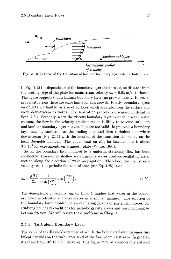
Fig. 2.16: Scheme of the transition of laminar boundary layer into turbulent one
In Fig. 2.15 the dependence of the boundary layer thickness, {;, on distance from
the leading edge of the plate for mainstream velocity Uo = 0.02 mis, is shown.
The figure suggests that a laminar boundary layer can grow endlessly. However,
in real situations there are some limits for this growth. Firstly, boundary layers
on objects are limited by size of vortices which separate from the surface and
move downstream as wakes. The separation process is discussed in detail in
Sect. 2.5.4. Secondly, when the viscous boundary layer extends into the water
column, the flow in the velocity gradient region is likely to become turbulent
and laminar boundary layer relationships are not valid. In practice, a boundary
layer may by laminar near the leading edge and then turbulent somewhere
downstream (Fig. 2.16) with the location of the transition depending on the
local Reynolds number. The upper limit on Rex for laminar flow is about
3 x 10 6 for experiments on a smooth plate (White, 1994).
So far the boundary layer induced by a uniform, stationary flow has been
considered. However in shallow water, gravity waves produce oscillating water
motion along the direction of wave propagation. Therefore, the mainstream
velocity, Un, is a periodic function of time (see Eq. 4.25), i.e.:
gHT 1
(21ft)
Uo = U cosh (2lh) cos T .
(2.50)
The dependence of velocity, Un, on time, t, implies that water in the boundary layer accelerates and decelerates in a similar manner. The solution of
the boundary layer problem in an oscillating flow is of particular interest for
studying boundary conditions for periodic gravity waves and wave damping by
bottom friction. We will revisit these problems in Chap. 4.
2.5.4 Turbulent Boundary Layer
The value of the Reynolds number at which the boundary layer becomes turbulent depends on the turbulence level of the free incoming stream. In general,
it ranges from 10 5 to 10 6 However, this figure may be considerably reduced
transition
/
laminar '
j/laminar sublayer
logarithmic profile
o/velocity
--. x
43
Fig. 2.16: Scheme of the transition of laminar boundary layer into turbulent one
In Fig. 2.15 the dependence of the boundary layer thickness, {;, on distance from
the leading edge of the plate for mainstream velocity Uo = 0.02 mis, is shown.
The figure suggests that a laminar boundary layer can grow endlessly. However,
in real situations there are some limits for this growth. Firstly, boundary layers
on objects are limited by size of vortices which separate from the surface and
move downstream as wakes. The separation process is discussed in detail in
Sect. 2.5.4. Secondly, when the viscous boundary layer extends into the water
column, the flow in the velocity gradient region is likely to become turbulent
and laminar boundary layer relationships are not valid. In practice, a boundary
layer may by laminar near the leading edge and then turbulent somewhere
downstream (Fig. 2.16) with the location of the transition depending on the
local Reynolds number. The upper limit on Rex for laminar flow is about
3 x 10 6 for experiments on a smooth plate (White, 1994).
So far the boundary layer induced by a uniform, stationary flow has been
considered. However in shallow water, gravity waves produce oscillating water
motion along the direction of wave propagation. Therefore, the mainstream
velocity, Un, is a periodic function of time (see Eq. 4.25), i.e.:
gHT 1
(21ft)
Uo = U cosh (2lh) cos T .
(2.50)
The dependence of velocity, Un, on time, t, implies that water in the boundary layer accelerates and decelerates in a similar manner. The solution of
the boundary layer problem in an oscillating flow is of particular interest for
studying boundary conditions for periodic gravity waves and wave damping by
bottom friction. We will revisit these problems in Chap. 4.
2.5.4 Turbulent Boundary Layer
The value of the Reynolds number at which the boundary layer becomes turbulent depends on the turbulence level of the free incoming stream. In general,
it ranges from 10 5 to 10 6 However, this figure may be considerably reduced