

26
2. Water at Rest and in Motion
Eulerian Method. In the Eulerian method, named after the Swiss-born mathematician Leonhard Euler (1707-1783), the velocity and pressure are computed
at a given point as functions of time:
u = h(x,y,z,t)
v=h(x,y,z,t)
w = h(x,y,z,t)
P = f4(x, y, z, t)
horizontal component of velocity
(parallel to x - axis),
horizontal component of velocity
(parallel to y-axis),
vertical component of velocity
pressure in fluid.
(2.14)
A simple example of these two different descriptions is the analysis of suspended sediment flow in an estuary. One investigator, located in the estuary, ignores specific sediment particles and measures their average velocity and
concentration as a function of time and position within the estuary. This investigator is using the Eulerian description of the sediment flow. The other
investigators may be interested in the path, speed and fate of specific sediments. They use the Lagrangian method.
2.3.2 Steady and Unsteady Flow
When flow is not time-dependent, the streamlines, pathlines and streaklines
are identical. This is know as steady flow. However, when the flow changes
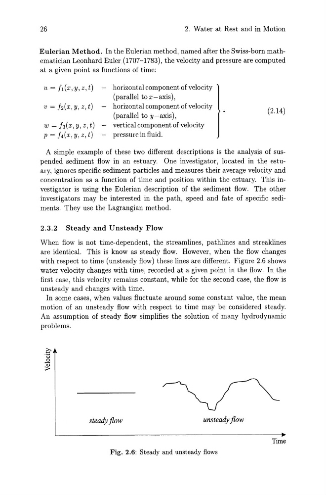
with respect to time (unsteady flow) these lines are different. Figure 2.6 shows
water velocity changes with time, recorded at a given point in the flow. In the
first case, this velocity remains constant, while for the second case, the flow is
unsteady and changes with time.
In some cases, when values fluctuate around some constant value, the mean
motion of an unsteady flow with respect to time may be considered steady.
An assumption of steady flow simplifies the solution of many hydrodynamic
problems .
. £ u o
~
steady flow
unsteady flow
Time
Fig. 2.6: Steady and unsteady flows
2. Water at Rest and in Motion
Eulerian Method. In the Eulerian method, named after the Swiss-born mathematician Leonhard Euler (1707-1783), the velocity and pressure are computed
at a given point as functions of time:
u = h(x,y,z,t)
v=h(x,y,z,t)
w = h(x,y,z,t)
P = f4(x, y, z, t)
horizontal component of velocity
(parallel to x - axis),
horizontal component of velocity
(parallel to y-axis),
vertical component of velocity
pressure in fluid.
(2.14)
A simple example of these two different descriptions is the analysis of suspended sediment flow in an estuary. One investigator, located in the estuary, ignores specific sediment particles and measures their average velocity and
concentration as a function of time and position within the estuary. This investigator is using the Eulerian description of the sediment flow. The other
investigators may be interested in the path, speed and fate of specific sediments. They use the Lagrangian method.
2.3.2 Steady and Unsteady Flow
When flow is not time-dependent, the streamlines, pathlines and streaklines
are identical. This is know as steady flow. However, when the flow changes
with respect to time (unsteady flow) these lines are different. Figure 2.6 shows
water velocity changes with time, recorded at a given point in the flow. In the
first case, this velocity remains constant, while for the second case, the flow is
unsteady and changes with time.
In some cases, when values fluctuate around some constant value, the mean
motion of an unsteady flow with respect to time may be considered steady.
An assumption of steady flow simplifies the solution of many hydrodynamic
problems .
. £ u o
~
steady flow
unsteady flow
Time
Fig. 2.6: Steady and unsteady flows