

334
9 Experimental Methods in Fluid Mechanics
9.5.4 Calculation of Statistical Characteristics of Waves
The basic statistical ocean flow parameters, namely surface displacement, waveinduced velocities and pressure as well as all kinds of turbulent oscillations, are
random variables subjected to various statistics which can be evaluated using
experimental data.
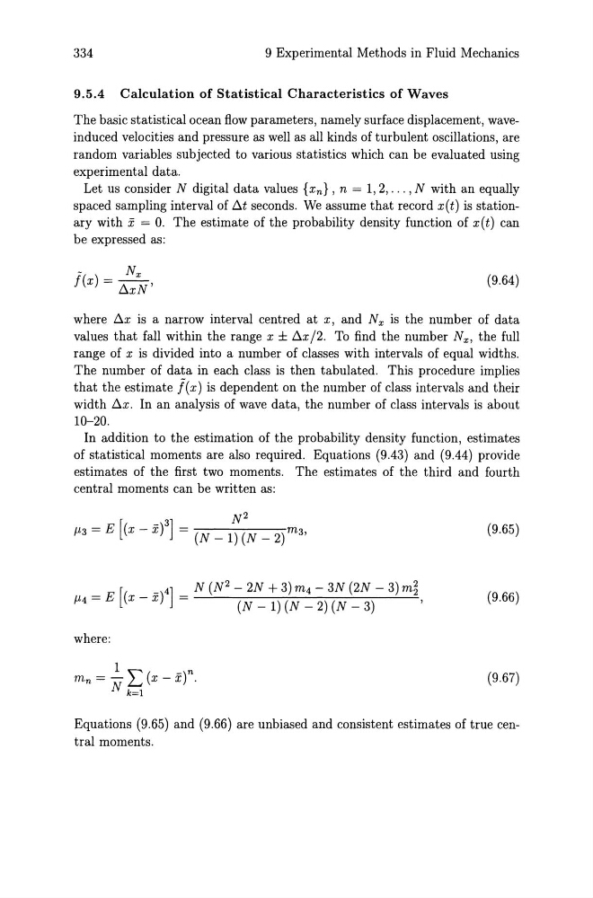
Let us consider N digital data values {x n } , n = 1,2, ... ,N with an equally
spaced sampling interval of !:::.t seconds. We assume that record x(t) is stationary with £ = O. The estimate of the probability density function of x(t) can
be expressed as:
-
N x
f(x) = !:::.xN'
(9.64)
where !:::.x is a narrow interval centred at x, and Nx is the number of data
values that fall within the range x ± !:::.x/2. To find the number Nx , the full
range of x is divided into a number of classes with intervals of equal widths.
The number of data in each class is then tabulated. This procedure implies
that the estimate j( x) is dependent on the number of class intervals and their
width !:::.x. In an analysis of wave data, the number of class intervals is about
10-20.
In addition to the estimation of the probability density function, estimates
of statistical moments are also required. Equations (9.43) and (9.44) provide
estimates of the first two moments. The estimates of the third and fourth
central moments can be written as:
(9.65)
= E [(x _ £)4] = N (N 2 - 2N + 3) m4 - 3N (2N - 3) m§
114
(N - 1) (N - 2) (N - 3)
,
(9.66)
where:
1 "
n
mn = N LJ (x - x) .
k=l
(9.67)
Equations (9.65) and (9.66) are unbiased and consistent estimates of true central moments.
9 Experimental Methods in Fluid Mechanics
9.5.4 Calculation of Statistical Characteristics of Waves
The basic statistical ocean flow parameters, namely surface displacement, waveinduced velocities and pressure as well as all kinds of turbulent oscillations, are
random variables subjected to various statistics which can be evaluated using
experimental data.
Let us consider N digital data values {x n } , n = 1,2, ... ,N with an equally
spaced sampling interval of !:::.t seconds. We assume that record x(t) is stationary with £ = O. The estimate of the probability density function of x(t) can
be expressed as:
-
N x
f(x) = !:::.xN'
(9.64)
where !:::.x is a narrow interval centred at x, and Nx is the number of data
values that fall within the range x ± !:::.x/2. To find the number Nx , the full
range of x is divided into a number of classes with intervals of equal widths.
The number of data in each class is then tabulated. This procedure implies
that the estimate j( x) is dependent on the number of class intervals and their
width !:::.x. In an analysis of wave data, the number of class intervals is about
10-20.
In addition to the estimation of the probability density function, estimates
of statistical moments are also required. Equations (9.43) and (9.44) provide
estimates of the first two moments. The estimates of the third and fourth
central moments can be written as:
(9.65)
= E [(x _ £)4] = N (N 2 - 2N + 3) m4 - 3N (2N - 3) m§
114
(N - 1) (N - 2) (N - 3)
,
(9.66)
where:
1 "
n
mn = N LJ (x - x) .
k=l
(9.67)
Equations (9.65) and (9.66) are unbiased and consistent estimates of true central moments.