

46
2. BasicFinite-Difference Methods
(a)
. . .
, ,
, ,
. , " 0 . 0
. ,
; ' - -0 - o · 0
(bl
,
,
0 '
0 ,'0
,
· 0 ,
,'0 ' 0
0
- - 0 , , - o· <) . 0 . 0
0
,
') ' 0 0 0 0
0
0
,
,
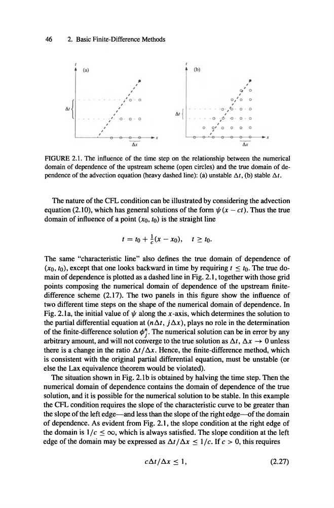
FIGURE 2.1. The influence of the time step on the relationship between the numerical
domain of dependence of the upstream scheme (open circles) and the true domain of dependence of the advection equation (heavy dashedline): (a) unstable St ; (b) stable ßt.
The nature of the CFL condition can be illustrated by considering the advection
equation (2.10), which has general solutions of the form 1/1 (x - ct). Thus the true
domain of inftuence of a point (xo, ro) is the straight line
t = to + l(x -xo),
e
t::: to.
The same "characteristic line" also defines the true domain of dependence of
(xo, to), except that one looks backward in time by requiring t ::: to. The true domain of dependence is plotted as a dashed line in Fig. 2.1, together with those grid
points composing the numerical domain of dependence of the upstream finitedifference scheme (2.17). The two panels in this figure show the inftuence of
two different time steps on the shape of the numerical domain of dependence. In
Fig. 2.1a, the initial value of 1/1 along the x -axis, which determines the solution to
the partial differential equation at (n t..t, j l:i.x), plays no role in the determination
of the finite-difference solution r/Jj. The numerical solution can be in error by any
arbitrary arnount, and will not converge to the true solution as l:i.t, l:i.x
0 unless
there is a change in the ratio l:i.t/ Sx, Hence, the finite-difference method, which
is consistent with the original partial differential equation, must be unstable (or
else the Lax equivalence theorem would be violated).
The situation shown in Fig . 2.1b is obtained by halving the time step. Then the
numerical domain of dependence contains the domain of dependence of the true
solution, and it is possible for the numerical solution to be stable. In this example
the CFL condition requires the slope of the characteristic curve to be greater than
the slope of the left edge-and less than the slope of the right edge-of the domain
of dependence. As evident from Fig. 2.1, the slope condition at the right edge of
the domain is 1/ c ::: 00, which is always satisfied . The slope condition at the left
edge of the domain may be expressed as l:i.t/ Sx ::: 1/c. If c > 0, this requires
cl:i.t/l:i.x::: I,
(2.27)
2. BasicFinite-Difference Methods
(a)
. . .
, ,
, ,
. , " 0 . 0
. ,
; ' - -0 - o · 0
(bl
,
,
0 '
0 ,'0
,
· 0 ,
,'0 ' 0
0
- - 0 , , - o· <) . 0 . 0
0
,
') ' 0 0 0 0
0
0
,
,
FIGURE 2.1. The influence of the time step on the relationship between the numerical
domain of dependence of the upstream scheme (open circles) and the true domain of dependence of the advection equation (heavy dashedline): (a) unstable St ; (b) stable ßt.
The nature of the CFL condition can be illustrated by considering the advection
equation (2.10), which has general solutions of the form 1/1 (x - ct). Thus the true
domain of inftuence of a point (xo, ro) is the straight line
t = to + l(x -xo),
e
t::: to.
The same "characteristic line" also defines the true domain of dependence of
(xo, to), except that one looks backward in time by requiring t ::: to. The true domain of dependence is plotted as a dashed line in Fig. 2.1, together with those grid
points composing the numerical domain of dependence of the upstream finitedifference scheme (2.17). The two panels in this figure show the inftuence of
two different time steps on the shape of the numerical domain of dependence. In
Fig. 2.1a, the initial value of 1/1 along the x -axis, which determines the solution to
the partial differential equation at (n t..t, j l:i.x), plays no role in the determination
of the finite-difference solution r/Jj. The numerical solution can be in error by any
arbitrary arnount, and will not converge to the true solution as l:i.t, l:i.x
0 unless
there is a change in the ratio l:i.t/ Sx, Hence, the finite-difference method, which
is consistent with the original partial differential equation, must be unstable (or
else the Lax equivalence theorem would be violated).
The situation shown in Fig . 2.1b is obtained by halving the time step. Then the
numerical domain of dependence contains the domain of dependence of the true
solution, and it is possible for the numerical solution to be stable. In this example
the CFL condition requires the slope of the characteristic curve to be greater than
the slope of the left edge-and less than the slope of the right edge-of the domain
of dependence. As evident from Fig. 2.1, the slope condition at the right edge of
the domain is 1/ c ::: 00, which is always satisfied . The slope condition at the left
edge of the domain may be expressed as l:i.t/ Sx ::: 1/c. If c > 0, this requires
cl:i.t/l:i.x::: I,
(2.27)