

430
8. Nonreflecting Boundary Conditions
may be written as
w m+ 1 _ wm
(pm+1 _ pm+1
N-!
N-! +
2
N-!
N-I +
pm _ pm
N
N - I
) = b m I _ U
N-,;
1
-,; ,
Bx
m
+
1 - w
(8.62)
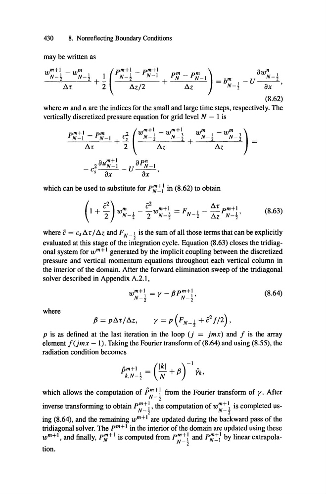
where m and n are the indices for the small and large time steps, respectively. The
vertically discretized pressure equation for grid level N - 1 is
_P,;..;.;:;_-..:..I_-_P,;..;.N_-..:..I + c;
+1
(W
m+1 + w
m
N -! - W
m
N -
)
2
ß m+1
ßpn
2 U N_ 1
N-I
-c - - - - U - - - ,
which can be used to substitute for
l in (8.62) to obtain
S
ßx
ßx
1 + -
(32) w m - _w m+ 1 = F
(32
J _ _
2
N-!
2
N -'j
(
pm+1
N-!'
(8.63)
where (3 =
r /
and F N
I is the sum of all those terms that can be explicitly
-'j
evaluated at this stage of the integration cycle. Equation (8.63) closes the tridiagonal system for w m +1 generated by the implicit coupling between the discretized
pressure and vertical momentum equations throughout each vertical column in
the interior of the domain. After the forward elimination sweep of the tridiagonal
solver described in Appendix A.2.1,
(8.64)
where
y=p(F N _!+(32f/2),
p is as defined at the last iteration in the 100p (j = jmx) and f is the array
element f(jmx - 1). Taking the Fourier transform of (8.64) and using (8.55), the
radiation condition becomes
ßm+1
k,N-1
=
N
ß)-I Yk,
which allows the computation of ßm+: from the Fourier transform of y. After
N- ,;
inverse transforming to obtain pm+: , the computation of
is completed usN -'j
N-,;
ing (8.64), and the remaining w m +I are updated during the backward pass of the
tridiagonal solver. The pm+I in the interior of the domain are updated using these
w m+ l , and finally, p;:;+1 is computed from pm+: and
by linear extrapolaN -,;
tion.
8. Nonreflecting Boundary Conditions
may be written as
w m+ 1 _ wm
(pm+1 _ pm+1
N-!
N-! +
2
N-!
N-I +
pm _ pm
N
N - I
) = b m I _ U
N-,;
1
-,; ,
Bx
m
+
1 - w
(8.62)
where m and n are the indices for the small and large time steps, respectively. The
vertically discretized pressure equation for grid level N - 1 is
_P,;..;.;:;_-..:..I_-_P,;..;.N_-..:..I + c;
+1
(W
m+1 + w
m
N -! - W
m
N -
)
2
ß m+1
ßpn
2 U N_ 1
N-I
-c - - - - U - - - ,
which can be used to substitute for
l in (8.62) to obtain
S
ßx
ßx
1 + -
(32) w m - _w m+ 1 = F
(32
J _ _
2
N-!
2
N -'j
(
pm+1
N-!'
(8.63)
where (3 =
r /
and F N
I is the sum of all those terms that can be explicitly
-'j
evaluated at this stage of the integration cycle. Equation (8.63) closes the tridiagonal system for w m +1 generated by the implicit coupling between the discretized
pressure and vertical momentum equations throughout each vertical column in
the interior of the domain. After the forward elimination sweep of the tridiagonal
solver described in Appendix A.2.1,
(8.64)
where
y=p(F N _!+(32f/2),
p is as defined at the last iteration in the 100p (j = jmx) and f is the array
element f(jmx - 1). Taking the Fourier transform of (8.64) and using (8.55), the
radiation condition becomes
ßm+1
k,N-1
=
N
ß)-I Yk,
which allows the computation of ßm+: from the Fourier transform of y. After
N- ,;
inverse transforming to obtain pm+: , the computation of
is completed usN -'j
N-,;
ing (8.64), and the remaining w m +I are updated during the backward pass of the
tridiagonal solver. The pm+I in the interior of the domain are updated using these
w m+ l , and finally, p;:;+1 is computed from pm+: and
by linear extrapolaN -,;
tion.