

(7.83)
(7.84)
(7.85)
368
7. Physically Insignificant Fast Waves
removed by the Asselin time filter (2.50), which is often used in conjunction with
leapfrog time-differencing to prevent the divergence of the solution on the odd and
even time steps. Other filtering techniques have also been suggested and will be
discussed after considering a partial-splitting approximation to the compressible
Boussinesq system.
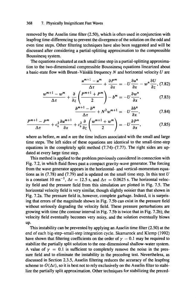
The equations evaluated at each small time step in a partial-splitting approximation to the two-dimensional compressible Boussinesq cquations Iinearized about
a basic-state flow with Brunt-Väisälä frequency N and horizontal velocity U are
u m + 1 _ um opm
ou n
su
- - - - + - - = - U -
w m+1 _ ui"
/),, :r
OX
m
OX - w
n _
, (7.82)
0 (pm+l + pm)
ow n
OZ
- - - - + -
-b = - U - ,
8.
OZ
2
OX
b m + 1 _ b"
obn
_ _ _ _ +N 2 w m + 1 = - U - ,
8.
pm+l _ pm
2 0um+ 1
2 0 (w m+ 1 + w m)
----+C --+c -
8.
s OX
s oz
2
OX
b
= -U-- ,
opn
where as before, m and n are the time indices associated with the sm all and large
time steps. The left sides of these equations are identical to the small-time-step
equations in the completely split method (7.74)-(7.77). The right sides are updated at every large time step.
This method is applied to the problem previously con sidered in connection with
Fig . 7.2, in which fluid flows past a compact gravity-wave generator. The forcing
from the wave generator appears in the horizontal- and vertical-momentum equations as in (7.78) and (7.79) and is updated on the small time step. In this test U
is a constant 10 ms", 81 = 12.5 s, and 8. = 0.0625 s. The horizontal velocity field and the pressure field from this simulation are plotted in Fig . 7.5 . The
horizontal velocity field is very similar, though slightly noisier than that shown in
Fig . 7.2a. The pressure field is, however, complete garbage. Indeed, it is surprising that errors of the magnitude shown in Fig . 7.5b can cxist in the pressure field
without seriously degrading the velocity field . These pressure perturbations are
growing with time (the contour interval in Fig . 7.5b is twice that in Fig. 7.2b); the
velocity field eventually becomes very noisy, and the solution eventually blows
up.
This instability can be prevented by applying an Assclin time filter (2.50) at the
end of each big-step-small-step integration cycle. Skamarock and Klemp (1992)
have shown that filtering coefficients on the order of y = 0.] may be required to
stabilize the partially split solution to the one-dimensional shallow-water system.
A value of y = 0 .] is sufficient to completely remove thc noise in the pressure field and to eliminate the instability in the preceding test. Nevertheless, as
discussed in Section 2.3.5, Asselin filtering reduces thc accuracy of the leapfrog
scheme to 0(81), so it is best not to rely exclusively on the Asselin filter to stabilize the partially split approximation. Other techniques for stabilizing the preced-
(7.84)
(7.85)
368
7. Physically Insignificant Fast Waves
removed by the Asselin time filter (2.50), which is often used in conjunction with
leapfrog time-differencing to prevent the divergence of the solution on the odd and
even time steps. Other filtering techniques have also been suggested and will be
discussed after considering a partial-splitting approximation to the compressible
Boussinesq system.
The equations evaluated at each small time step in a partial-splitting approximation to the two-dimensional compressible Boussinesq cquations Iinearized about
a basic-state flow with Brunt-Väisälä frequency N and horizontal velocity U are
u m + 1 _ um opm
ou n
su
- - - - + - - = - U -
w m+1 _ ui"
/),, :r
OX
m
OX - w
n _
, (7.82)
0 (pm+l + pm)
ow n
OZ
- - - - + -
-b = - U - ,
8.
OZ
2
OX
b m + 1 _ b"
obn
_ _ _ _ +N 2 w m + 1 = - U - ,
8.
pm+l _ pm
2 0um+ 1
2 0 (w m+ 1 + w m)
----+C --+c -
8.
s OX
s oz
2
OX
b
= -U-- ,
opn
where as before, m and n are the time indices associated with the sm all and large
time steps. The left sides of these equations are identical to the small-time-step
equations in the completely split method (7.74)-(7.77). The right sides are updated at every large time step.
This method is applied to the problem previously con sidered in connection with
Fig . 7.2, in which fluid flows past a compact gravity-wave generator. The forcing
from the wave generator appears in the horizontal- and vertical-momentum equations as in (7.78) and (7.79) and is updated on the small time step. In this test U
is a constant 10 ms", 81 = 12.5 s, and 8. = 0.0625 s. The horizontal velocity field and the pressure field from this simulation are plotted in Fig . 7.5 . The
horizontal velocity field is very similar, though slightly noisier than that shown in
Fig . 7.2a. The pressure field is, however, complete garbage. Indeed, it is surprising that errors of the magnitude shown in Fig . 7.5b can cxist in the pressure field
without seriously degrading the velocity field . These pressure perturbations are
growing with time (the contour interval in Fig . 7.5b is twice that in Fig. 7.2b); the
velocity field eventually becomes very noisy, and the solution eventually blows
up.
This instability can be prevented by applying an Assclin time filter (2.50) at the
end of each big-step-small-step integration cycle. Skamarock and Klemp (1992)
have shown that filtering coefficients on the order of y = 0.] may be required to
stabilize the partially split solution to the one-dimensional shallow-water system.
A value of y = 0 .] is sufficient to completely remove thc noise in the pressure field and to eliminate the instability in the preceding test. Nevertheless, as
discussed in Section 2.3.5, Asselin filtering reduces thc accuracy of the leapfrog
scheme to 0(81), so it is best not to rely exclusively on the Asselin filter to stabilize the partially split approximation. Other techniques for stabilizing the preced-