

6.1 The Scalar Advection Equation
311
(6.16) into (6.8) to obtain
t/I'r
l = t/ld+D.t(:t
+O[{D.t)2J
= v« + 0 [{D.t)2].
(6.17)
According to (6.13) the contribution from the trajectory calcu1ation to the global
truncation error in the semi-Lagrangian scheme is ( t/lj+I - t/ld) / D.t, so the error
generated by the Euler method is 0 (M) .
A second-order-accurate result can be obtained using the two-stage trajectory
calculation
x, = x n+1 - u{x n+ l , t n)D.t/2,
xl! = x n+ 1 - u{x*, tn+!)D.t .
J
(6.18)
(6.19)
As before, the initial condition is x n +I = X i: This differs slightly from the classical Runge-Kutta midpoint method discussed in Section 2.3.3 in that the first
stage uses the velocity u(x n+l , t") rather than u{x n+l , t n+I ) ; the 1atter is more
convenient if u n+ I is being predicted at the same time as
I . The second-order
accuracy of this calculation can be verified as folIows. Substitute (6.18) into (6.19)
and let the superscript n + 1 denote evaluation at (x{t n+ I ) , t n+I ) . Then
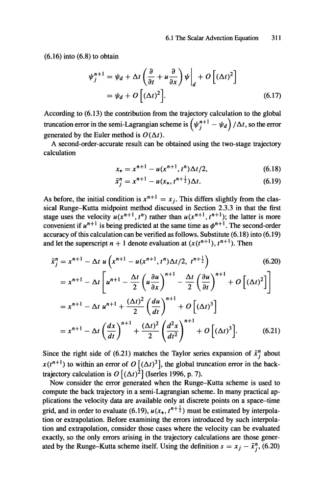
Since the right side of (6.21) matches the Taylor series expansion of xj about
x {t n +
l ) to within an error of 0 [CD.t)3], the global truncation error in the backtrajectory calculation is 0 [(D.t)2] (Iserles 1996, p. 7).
Now consider the error generated when the Runge-Kutta scheme is used to
compute the back trajectory in a semi-Lagrangian scheme. In many practical applications the velocity data are available only at discrete points on a space-time
grid, and in order to eva1uate (6.19), u{x*, t n+!) must be estimated by interpolation or extrapolation. Before examining the errors introduced by such interpolation and extrapolation, consider those cases where the velocity can be eva1uated
exactly, so the only errors arising in the trajectory calculations are those generated by the Runge-Kutta scheme itself. Using the definition s = x j - xj , (6.20)
311
(6.16) into (6.8) to obtain
t/I'r
l = t/ld+D.t(:t
+O[{D.t)2J
= v« + 0 [{D.t)2].
(6.17)
According to (6.13) the contribution from the trajectory calcu1ation to the global
truncation error in the semi-Lagrangian scheme is ( t/lj+I - t/ld) / D.t, so the error
generated by the Euler method is 0 (M) .
A second-order-accurate result can be obtained using the two-stage trajectory
calculation
x, = x n+1 - u{x n+ l , t n)D.t/2,
xl! = x n+ 1 - u{x*, tn+!)D.t .
J
(6.18)
(6.19)
As before, the initial condition is x n +I = X i: This differs slightly from the classical Runge-Kutta midpoint method discussed in Section 2.3.3 in that the first
stage uses the velocity u(x n+l , t") rather than u{x n+l , t n+I ) ; the 1atter is more
convenient if u n+ I is being predicted at the same time as
I . The second-order
accuracy of this calculation can be verified as folIows. Substitute (6.18) into (6.19)
and let the superscript n + 1 denote evaluation at (x{t n+ I ) , t n+I ) . Then
Since the right side of (6.21) matches the Taylor series expansion of xj about
x {t n +
l ) to within an error of 0 [CD.t)3], the global truncation error in the backtrajectory calculation is 0 [(D.t)2] (Iserles 1996, p. 7).
Now consider the error generated when the Runge-Kutta scheme is used to
compute the back trajectory in a semi-Lagrangian scheme. In many practical applications the velocity data are available only at discrete points on a space-time
grid, and in order to eva1uate (6.19), u{x*, t n+!) must be estimated by interpolation or extrapolation. Before examining the errors introduced by such interpolation and extrapolation, consider those cases where the velocity can be eva1uated
exactly, so the only errors arising in the trajectory calculations are those generated by the Runge-Kutta scheme itself. Using the definition s = x j - xj , (6.20)