

5.7 Two Spatial Dimensions
279
(a)
(b)
(c)
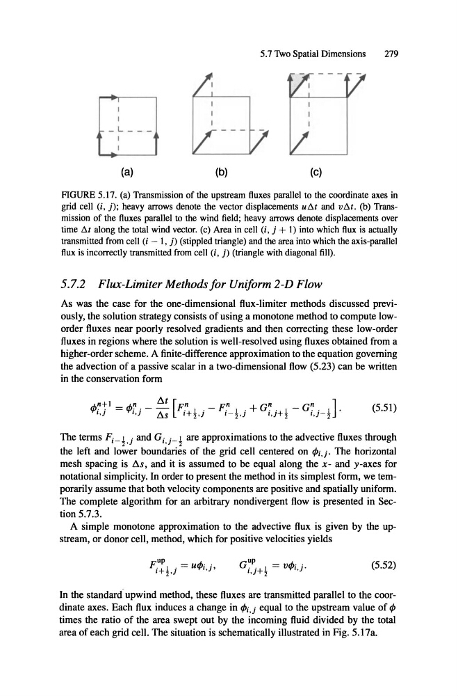
FIGURE 5.17 . (a) Transmission of the upstream fluxes parallel to the eoordinate axes in
grid eell (i, j); heavy arrows denote the veetor displaeements u S: and vtlt. (b) Transmission of the fluxes parallel to the wind field; heavy arrows denote displaeements over
time tlt along the total wind veetor. (e) Area in eell (i, j + 1) into whieh flux is aetually
transmitted from eell (i - I, j) (stippled triangle) and the area into whieh the axis-parallel
flux is ineorreetly transmitted from eell (i, j) (triangle with diagonal fill).
5.7.2 Flux-Limiter Methodsfor Uniform 2-D Flow
As was the case for the one-dimensional flux-limiter methods discussed previously, the solution strategy consists of using a monotone method to compute loworder fluxes near poorly resolved gradients and then correcting these low-order
fluxes in regions where the solution is well-resolved using fluxes obtained from a
higher-order scheme. A finite-difference approximation to the equation goveming
the advection of a passive scalar in a two-dimensional flow (5.23) can be written
in the conservation form
Il s
Ilt
1
I
2')
, -
1 ,+
1- 2 ,)
I ,)
'+ 1 -
2
I ]
1')-2
'
(5.51)
The terms
and
are approximations to the advective fluxes through
the left and lower boundaries of the grid cell centered on
notational simplicity. In order to present the method in its simplest form, we temporarily assume that both velocity components are positive and spatially uniform .
The complete algorithm for an arbitrary nondivergent flow is presented in Section 5.7.3.
A simple monotone approximation to the advective flux is given by the upstream , or donor cell, method, which for positive velocities yields
up
F.+ 1 , = U
up
G , '+ 1 = V
(5.52)
In the standard upwind method, these fluxes are transmitted parallel to the coordinate axes. Each flux induces a change in
279
(a)
(b)
(c)
FIGURE 5.17 . (a) Transmission of the upstream fluxes parallel to the eoordinate axes in
grid eell (i, j); heavy arrows denote the veetor displaeements u S: and vtlt. (b) Transmission of the fluxes parallel to the wind field; heavy arrows denote displaeements over
time tlt along the total wind veetor. (e) Area in eell (i, j + 1) into whieh flux is aetually
transmitted from eell (i - I, j) (stippled triangle) and the area into whieh the axis-parallel
flux is ineorreetly transmitted from eell (i, j) (triangle with diagonal fill).
5.7.2 Flux-Limiter Methodsfor Uniform 2-D Flow
As was the case for the one-dimensional flux-limiter methods discussed previously, the solution strategy consists of using a monotone method to compute loworder fluxes near poorly resolved gradients and then correcting these low-order
fluxes in regions where the solution is well-resolved using fluxes obtained from a
higher-order scheme. A finite-difference approximation to the equation goveming
the advection of a passive scalar in a two-dimensional flow (5.23) can be written
in the conservation form
Il s
Ilt
1
I
2')
, -
1 ,+
1- 2 ,)
I ,)
'+ 1 -
2
I ]
1')-2
'
(5.51)
The terms
and
are approximations to the advective fluxes through
the left and lower boundaries of the grid cell centered on
notational simplicity. In order to present the method in its simplest form, we temporarily assume that both velocity components are positive and spatially uniform .
The complete algorithm for an arbitrary nondivergent flow is presented in Section 5.7.3.
A simple monotone approximation to the advective flux is given by the upstream , or donor cell, method, which for positive velocities yields
up
F.+ 1 , = U
up
G , '+ 1 = V
(5.52)
In the standard upwind method, these fluxes are transmitted parallel to the coordinate axes. Each flux induces a change in