

Problems
239
(b) Now retry the solution with 128 Fourier modes and compare your results with those obtained in (a) and, if available, with the finite-difference
solutions computed for Problem 13 of Chapter 3.
17. *Compute chapeau-function finite-element method solutions to Problem 16
using the previously specified numerical parameters. Try spatial resolutions
of ßx = -b and Sx = d4. If aj is the amplitude at the jth node, the
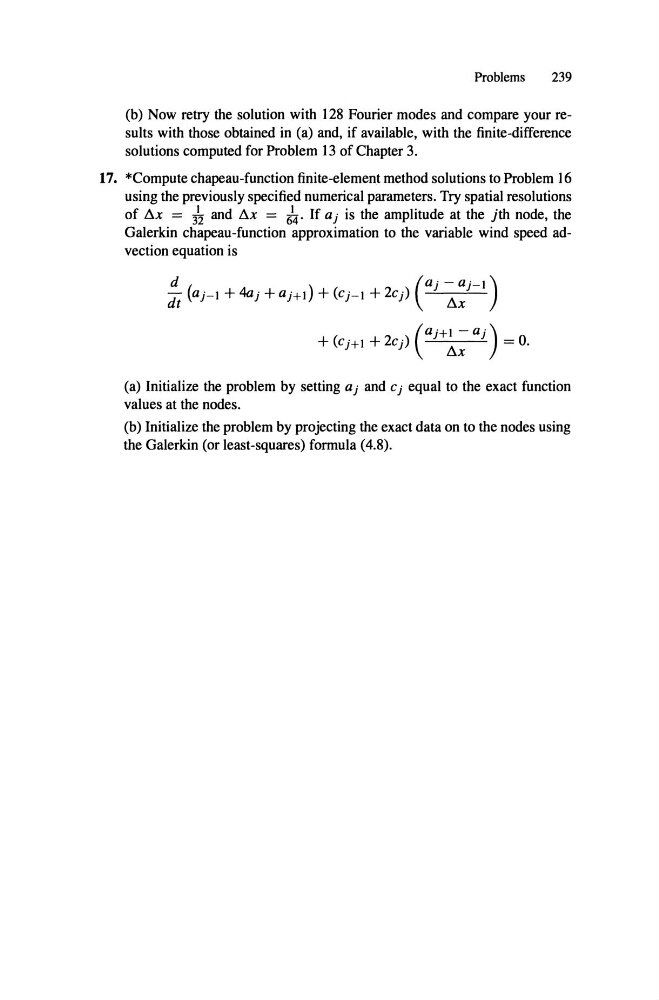
Galerkin chapeau-function approximation to the variable wind speed advection equation is
(a) Initialize the problem by setting a j and Cj equal to the exact function
values at the nodes.
(b) Initialize the problem by projecting the exact data on to the nodes using
the Galerkin (or least-squares) formula (4.8).
239
(b) Now retry the solution with 128 Fourier modes and compare your results with those obtained in (a) and, if available, with the finite-difference
solutions computed for Problem 13 of Chapter 3.
17. *Compute chapeau-function finite-element method solutions to Problem 16
using the previously specified numerical parameters. Try spatial resolutions
of ßx = -b and Sx = d4. If aj is the amplitude at the jth node, the
Galerkin chapeau-function approximation to the variable wind speed advection equation is
(a) Initialize the problem by setting a j and Cj equal to the exact function
values at the nodes.
(b) Initialize the problem by projecting the exact data on to the nodes using
the Galerkin (or least-squares) formula (4.8).