

4.4 Spherical Hannonics
latitude-Iongitude grid can be computed using the relation
M
1{!(A , J-L) = L am(J-L)e
im\
m=-M
203
(4.55)
am(J-L) = N(m) L am,nPm,n(J-L).
n=lml
where
(4.56)
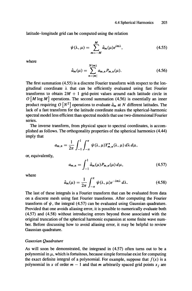
The first summation (4.55) is a discrete Fourier transform with respect to the longitudinal coordinate A that can be efficiently evaluated using fast Fourier
transforms to obtain 2M + I grid-point values around each latitude circle in
o [M log M] operations. The second summation (4.56) is essentially an inner
product requiring 0 [N 2 ] operations to evaluate a m at N different latitudes. The
lack of a fast transform for the latitude coordinate makes the spherical-harmonic
spectral modelless efficient than spectral models that use two-dimensional Fourier
series .
imply that
The inverse transform, from physical space to spectral coordinates, is accom7f
plished as follows. The orthogonality properties of the spherical harmonics (4.44)
am,n = -
1{!(A, J-L)Y:Z,n (A , J-L) d): dJ-L,
21r -\ -7f
I 1\1
or, equivalently,
(4.57)
where
(4.58)
The last of these integrals is a Fourier transform that can be evaluated from data
on a discrete mesh using fast Fourier transforms. After computing the Fourier
transform of 1{!, the integral (4.57) can be evaluated using Gaussian quadrature.
Provided that one avoids aliasing error, it is possible to numerically evaluate both
(4.57) and (4.58) without introducing errors beyond those associated with the
original truncation of the spherical harmonic expansion at some finite wave number. Before discussing how to avoid aliasing error, it may be helpful to review
Gaussian quadrature.
Gaussian Quadrature
As will soon be demonstrated, the integrand in (4.57) often turns out to be a
polynomial in J-L, which is fortuitous, because simple formulae exist for computing
the exact definite integral of a polynomial. For example, suppose that !(x) is a
latitude-Iongitude grid can be computed using the relation
M
1{!(A , J-L) = L am(J-L)e
im\
m=-M
203
(4.55)
am(J-L) = N(m) L am,nPm,n(J-L).
n=lml
where
(4.56)
The first summation (4.55) is a discrete Fourier transform with respect to the longitudinal coordinate A that can be efficiently evaluated using fast Fourier
transforms to obtain 2M + I grid-point values around each latitude circle in
o [M log M] operations. The second summation (4.56) is essentially an inner
product requiring 0 [N 2 ] operations to evaluate a m at N different latitudes. The
lack of a fast transform for the latitude coordinate makes the spherical-harmonic
spectral modelless efficient than spectral models that use two-dimensional Fourier
series .
imply that
The inverse transform, from physical space to spectral coordinates, is accom7f
plished as follows. The orthogonality properties of the spherical harmonics (4.44)
am,n = -
1{!(A, J-L)Y:Z,n (A , J-L) d): dJ-L,
21r -\ -7f
I 1\1
or, equivalently,
(4.57)
where
(4.58)
The last of these integrals is a Fourier transform that can be evaluated from data
on a discrete mesh using fast Fourier transforms. After computing the Fourier
transform of 1{!, the integral (4.57) can be evaluated using Gaussian quadrature.
Provided that one avoids aliasing error, it is possible to numerically evaluate both
(4.57) and (4.58) without introducing errors beyond those associated with the
original truncation of the spherical harmonic expansion at some finite wave number. Before discussing how to avoid aliasing error, it may be helpful to review
Gaussian quadrature.
Gaussian Quadrature
As will soon be demonstrated, the integrand in (4.57) often turns out to be a
polynomial in J-L, which is fortuitous, because simple formulae exist for computing
the exact definite integral of a polynomial. For example, suppose that !(x) is a