

192
4. Series-Expansion Methods
The grid-point nature of the pseudospectral method is apparent in (4.37), which
is similar to the time-tendency equations" that arise in differential-difference approximations to the advection equation, except that the derivative is computed in a
special way. Instead of using finite differences , the spatial derivative is calculated
at each time step by first computing the Fourier coefficients through the discrete
Fourier transform
then differentiating each Fourier mode analytically and inverse transfonning according to (4.38). This procedure requires two fast Fourier transfonns (FFf) per
time step .
The advantage of the pseudospectral method relative to conventional finitedifference schemes is that provided the solution is smooth, the pseudospectral
method is more accurate. As discussed in Section 3.2.1, the error in the Fourier approximation to the derivative of an infinitely differentiable function will decrease
more rapidly than any finite power of S x as the grid resolution is increased . Thus,
like the spectral method, the pseudospectral method is essentially an infinite-order
finite-difference scheme. The disadvantage of the pseudospectral method is that it
requires more computation than conventional finite-difference schemes when both
methods are used with the same spatial resolution. If M is the total number of grid
points, the FFfs in the pseudospectral computation require O(M 10g(M» operations per time step, whereas conventional finite-difference methods need only
O(M) operations. The extra work per time step may, however, be easily offset if
the increased accuracy of the pseudospectral representation allows the computations to be perfonned on a coarser mesh.
The advantage of the pseudospectral method relative to the spectral method is
that the pseudospectral method requires less computation. The increase in efficiency of the pseudospectral method is achieved by allowing aliasing error in the
computation of the products of spatially varying functions. As a consequence of
this aliasing error, the residual need not be orthogonal to the individual expan -
sion functions, and the pseudospectral method does not possess the conservation
properties discussed in Section 4.2.3. In particular, the pseudospectral method is
subject to nonlinear instability.
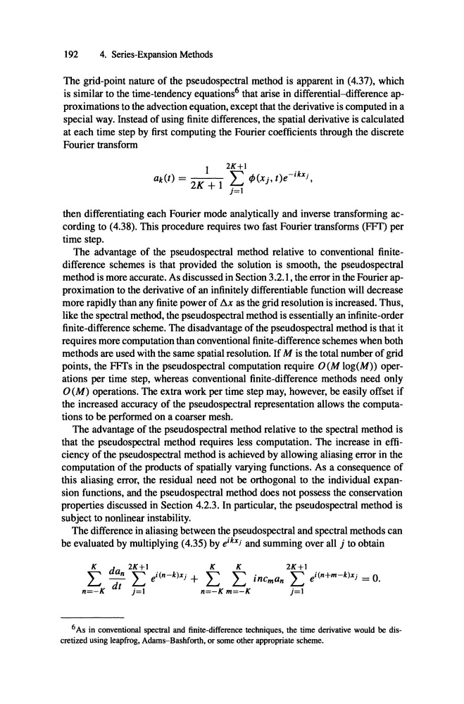
The difference in aliasing between the pseudospectral and spectral methods can
be evaluated by multiplying (4.35) by e i kx j and summing over all j to obtain
L
K
d
an
2K +I
L ei(n-k)xj + L
K
L
K
incma n
2K +I
L ei(n+m-k)xj = O.
n=-K dt j = 1
n=-K m=-K
j=1
6As in conventional spectral and finite-difference techniques, the time derivative would be discretized using leapfrog, Adams-Bashforth, or some other appropriate scheme.
4. Series-Expansion Methods
The grid-point nature of the pseudospectral method is apparent in (4.37), which
is similar to the time-tendency equations" that arise in differential-difference approximations to the advection equation, except that the derivative is computed in a
special way. Instead of using finite differences , the spatial derivative is calculated
at each time step by first computing the Fourier coefficients through the discrete
Fourier transform
then differentiating each Fourier mode analytically and inverse transfonning according to (4.38). This procedure requires two fast Fourier transfonns (FFf) per
time step .
The advantage of the pseudospectral method relative to conventional finitedifference schemes is that provided the solution is smooth, the pseudospectral
method is more accurate. As discussed in Section 3.2.1, the error in the Fourier approximation to the derivative of an infinitely differentiable function will decrease
more rapidly than any finite power of S x as the grid resolution is increased . Thus,
like the spectral method, the pseudospectral method is essentially an infinite-order
finite-difference scheme. The disadvantage of the pseudospectral method is that it
requires more computation than conventional finite-difference schemes when both
methods are used with the same spatial resolution. If M is the total number of grid
points, the FFfs in the pseudospectral computation require O(M 10g(M» operations per time step, whereas conventional finite-difference methods need only
O(M) operations. The extra work per time step may, however, be easily offset if
the increased accuracy of the pseudospectral representation allows the computations to be perfonned on a coarser mesh.
The advantage of the pseudospectral method relative to the spectral method is
that the pseudospectral method requires less computation. The increase in efficiency of the pseudospectral method is achieved by allowing aliasing error in the
computation of the products of spatially varying functions. As a consequence of
this aliasing error, the residual need not be orthogonal to the individual expan -
sion functions, and the pseudospectral method does not possess the conservation
properties discussed in Section 4.2.3. In particular, the pseudospectral method is
subject to nonlinear instability.
The difference in aliasing between the pseudospectral and spectral methods can
be evaluated by multiplying (4.35) by e i kx j and summing over all j to obtain
L
K
d
an
2K +I
L ei(n-k)xj + L
K
L
K
incma n
2K +I
L ei(n+m-k)xj = O.
n=-K dt j = 1
n=-K m=-K
j=1
6As in conventional spectral and finite-difference techniques, the time derivative would be discretized using leapfrog, Adams-Bashforth, or some other appropriate scheme.