

3.4 Diffusion, Sourees, and Sinks
145
time grid , but this may generate excessive noise in the numerical solution. One
should make a distinction between the shortest scale present on the numerical
mesh and the shortest scale at which the finite-difference scheme can be expected
to yield physically meaningful results. The accuracy of the solution is generally
not improved by applying forcing at wavelengths too short to be adequately simulated by the numerical scheme. Since almost all numerical methods do a very poor
job of simulating
waves and
oscillations, it is usually unwise to include
spatial and temporal scales in s(x, t) corresponding to wavelengths shorter than
about
or periods shorter than about
The optimal cutoff depends on the
numerical scheme and the nature of the problem being approximated. See Lander
and Hoskins (1997) for an example in which a cutoff wave number is determined
for extemal forcing in a spectral model of the Earth 's atmosphere.
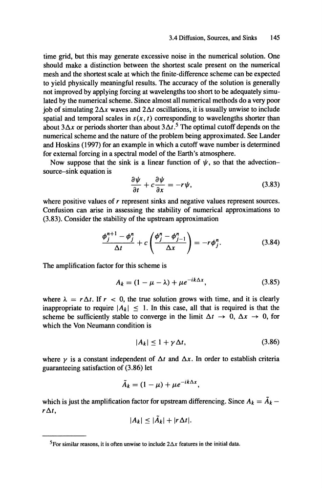
Now suppose that the sink is a linear function of 1{!, so that the advectionsource-sink equation is
a1{!
-
at
a1{!
+ c - = -r1{!,
ax
(3.83)
where positive values of r represent sinks and negative values represent sourees.
Confusion can arise in assessing the stability of numerical approximations to
(3.83). Consider the stability of the upstream approximation
(3.84)
The amplification factor for this scheme is
(3.85)
where ). = r
If r < 0, the true solution grows with time, and it is clearly
inappropriate to require IAk I :5 I. In this case, all that is required is that the
scheme be sufficiently stable to converge in the limit
which the Von Neumann condition is
0, Sx
0, for
(3.86)
where y is a constant independent of ßt and Sx, In order to establish criteria
guaranteeing satisfaction of (3.86) let
Ä k = (I - /L) + /Le- ik/,;x,
which is just the amplification factor for upstream differencing. Since Ak = Ä k -
r tst ,
5 For similar reasons , it is often unwise to include 2!'>.x features in the initial data.
145
time grid , but this may generate excessive noise in the numerical solution. One
should make a distinction between the shortest scale present on the numerical
mesh and the shortest scale at which the finite-difference scheme can be expected
to yield physically meaningful results. The accuracy of the solution is generally
not improved by applying forcing at wavelengths too short to be adequately simulated by the numerical scheme. Since almost all numerical methods do a very poor
job of simulating
waves and
oscillations, it is usually unwise to include
spatial and temporal scales in s(x, t) corresponding to wavelengths shorter than
about
or periods shorter than about
The optimal cutoff depends on the
numerical scheme and the nature of the problem being approximated. See Lander
and Hoskins (1997) for an example in which a cutoff wave number is determined
for extemal forcing in a spectral model of the Earth 's atmosphere.
Now suppose that the sink is a linear function of 1{!, so that the advectionsource-sink equation is
a1{!
-
at
a1{!
+ c - = -r1{!,
ax
(3.83)
where positive values of r represent sinks and negative values represent sourees.
Confusion can arise in assessing the stability of numerical approximations to
(3.83). Consider the stability of the upstream approximation
(3.84)
The amplification factor for this scheme is
(3.85)
where ). = r
If r < 0, the true solution grows with time, and it is clearly
inappropriate to require IAk I :5 I. In this case, all that is required is that the
scheme be sufficiently stable to converge in the limit
which the Von Neumann condition is
0, Sx
0, for
(3.86)
where y is a constant independent of ßt and Sx, In order to establish criteria
guaranteeing satisfaction of (3.86) let
Ä k = (I - /L) + /Le- ik/,;x,
which is just the amplification factor for upstream differencing. Since Ak = Ä k -
r tst ,
5 For similar reasons , it is often unwise to include 2!'>.x features in the initial data.