

3.2 Three or More Independent Variables
121
1.2
1.0
Q:)
0.6 ---s::
..................
"""' \.>
.........
*\.>
0.6
-----. .... ,""
,
.... ... ---, , \ \
'e;;
E
I
(a)
......
., \ \
\ :
\
4 _
6 -,
" "
--....... "
\ \
(b)
- .
I
,
0.2
.:
0.4
\
\ \
I
I
3
I
4 6
J
s:">,
'-'"
0
I
I
I
\
o 0.2 0.4 0.6 0.8 1.0 1.2 0 0.2 0.4 0.6 0.8 1.0 1.2
(c* jc) cosB
(c" jc) cosB
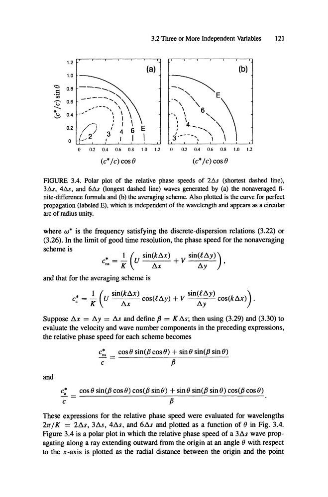
FlGDRE 3.4. Polar plot of the relative phase speeds of 2t1s (shortest dashed Une),
3t1s, 4t1s, and 6t1s (Iongest dashed Une) waves generated by (a) the nonaveraged finite-difference formula and (b) the averaging scheme. Also plotted is the curve for perfect
propagation (Iabeled E), which is independent of the wavelength and appears as a circular
arc of radius unity.
where to" is the frequency satisfying the discrete-dispersion relations (3.22) or
(3.26). In the limit of good time resolution, the phase speed for the nonaveraging
, "
scheme is
* _
co. - K
(Sin(kßX)
ßx
+ V
U
Sin(lßY») ,
ßy
and that for the averaging scheme is
I ( U
sin(kßx) cos(lßy) + V
S i n ( l ß Y » )
cos(kßx) .
ßy
c: = -
K
ßx
Suppose ßx = ßy = ßs and define ß = K ßs; then using (3.29) and (3.30) to
evaluate the velocity and wave number components in the preceding expressions,
the relative phase speed for each scheme becomes
c:. cos B sin(ß cos B) + sin B sin(ß sin B)
- =
and
c*
c
ß
cos B sin(ß cos B) cos(ß sin B) + sin B sin(ß sin B) cos(ß cos B)
--!!.. = -----'-----"--------"-----......:...--C
ß
These expressions for the relative phase speed were evaluated for wavelengths
2rrj K = 2ßs, 3ßs, 4ßs, and
and plotted as a function of e in Fig. 3.4.
Figure 3.4 is a polar plot in which the relative phase speed of a 3ßs wave propagating along a ray extending outward from the origin at an angle ewith respect
to the x -axis is plotted as the radial distance between the origin and the point
121
1.2
1.0
Q:)
0.6 ---s::
..................
"""' \.>
.........
*\.>
0.6
-----. .... ,""
,
.... ... ---, , \ \
'e;;
E
I
(a)
......
., \ \
\ :
\
4 _
6 -,
" "
--....... "
\ \
(b)
- .
I
,
0.2
.:
0.4
\
\ \
I
I
3
I
4 6
J
s:">,
'-'"
0
I
I
I
\
o 0.2 0.4 0.6 0.8 1.0 1.2 0 0.2 0.4 0.6 0.8 1.0 1.2
(c* jc) cosB
(c" jc) cosB
FlGDRE 3.4. Polar plot of the relative phase speeds of 2t1s (shortest dashed Une),
3t1s, 4t1s, and 6t1s (Iongest dashed Une) waves generated by (a) the nonaveraged finite-difference formula and (b) the averaging scheme. Also plotted is the curve for perfect
propagation (Iabeled E), which is independent of the wavelength and appears as a circular
arc of radius unity.
where to" is the frequency satisfying the discrete-dispersion relations (3.22) or
(3.26). In the limit of good time resolution, the phase speed for the nonaveraging
, "
scheme is
* _
co. - K
(Sin(kßX)
ßx
+ V
U
Sin(lßY») ,
ßy
and that for the averaging scheme is
I ( U
sin(kßx) cos(lßy) + V
S i n ( l ß Y » )
cos(kßx) .
ßy
c: = -
K
ßx
Suppose ßx = ßy = ßs and define ß = K ßs; then using (3.29) and (3.30) to
evaluate the velocity and wave number components in the preceding expressions,
the relative phase speed for each scheme becomes
c:. cos B sin(ß cos B) + sin B sin(ß sin B)
- =
and
c*
c
ß
cos B sin(ß cos B) cos(ß sin B) + sin B sin(ß sin B) cos(ß cos B)
--!!.. = -----'-----"--------"-----......:...--C
ß
These expressions for the relative phase speed were evaluated for wavelengths
2rrj K = 2ßs, 3ßs, 4ßs, and
and plotted as a function of e in Fig. 3.4.
Figure 3.4 is a polar plot in which the relative phase speed of a 3ßs wave propagating along a ray extending outward from the origin at an angle ewith respect
to the x -axis is plotted as the radial distance between the origin and the point