

2.6 Summary Discussion of Elementary Methods
99
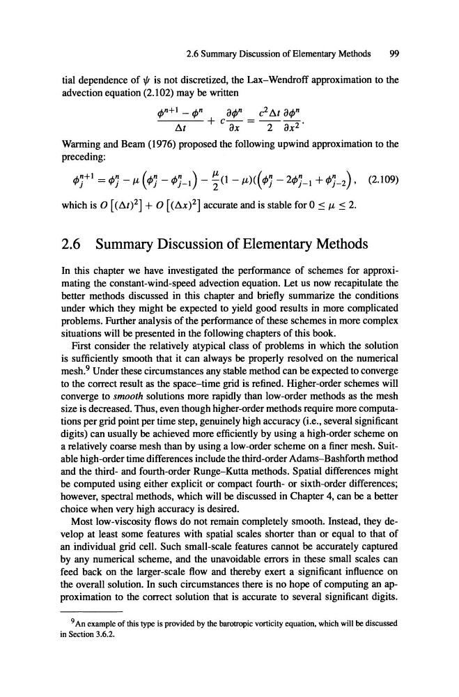
tial dependence of 1/1 is not discretized, the Lax-Wendroff approximation to the
advection equation (2.102) may be written
C Z/).( oifJn
ifJn+1 - ifJn
oifJn
.:..-------:.- + c - = - - - - .
Ilt
ox
2 ox z
Warming and Beam (1976) proposed the following upwind approximation to the
preceding :
ifJ'j+1 =ifJ'j -JL(ifJ'j -ifJ'j-I) -
-2ifJ'j_1 +ifJ'j-z) , (2.109)
which is 0 [(llt)Z] + 0 [(llx)Z] accurate and is stable for 0 ::s JL ::s 2.
2.6 Summary Discussion of Elementary Methods
In this chapter we have investigated the performance of schemes for approximating the constant-wind-speed advection equation . Let us now recapitulate the
better methods discussed in this chapter and briefly summarize the conditions
under which they might be expected to yield good results in more complicated
problems. Further analysis of the performance of these schemes in more complex
situations will be presented in the following chapters of this book.
First consider the relatively atypical dass of problems in which the solution
is sufficiently smooth that it can always be properly resolved on the numerical
mesh.? Under these circumstances any stable method can be expected to converge
to the correct result as the space-time grid is refined. Higher-order schemes will
converge to smooth solutions more rapidly than low-order methods as the mesh
size is decreased. Thus, even though higher-order methods require more computations per grid point per time step, genuinely high accuracy (i.e., several significant
digits) can usually be achieved more efficiently by using a high-order scheme on
a relatively coarse mesh than by using a low-order scheme on a finer mesh. Suitable high-order time differences include the third-order Adams-Bashforth method
and the third- and fourth-order Runge-Kutta methods. Spatial differences might
be computed using either explicit or compact fourth - or sixth-order differences ;
however, spectral methods, which will be discussed in Chapter 4, can be a better
choice when very high accuracy is desired.
Most low-viscosity flows do not remain completely smooth . Instead, they develop at least some features with spatial scales shorter than or equal to that of
an individual grid cell. Such small-scale features cannot be accurately captured
by any numerical scherne, and the unavoidable errors in these small scales can
feed back on the larger-scale flow and thereby exert a significant influence on
the overall solution. In such circumstances there is no hope of computing an approximation to the correct solution that is accurate to several significant digits.
9An exarnpleof this type is provided by the barotropicvorticity equation, which will be discussed
in Section 3.6.Z.
99
tial dependence of 1/1 is not discretized, the Lax-Wendroff approximation to the
advection equation (2.102) may be written
C Z/).( oifJn
ifJn+1 - ifJn
oifJn
.:..-------:.- + c - = - - - - .
Ilt
ox
2 ox z
Warming and Beam (1976) proposed the following upwind approximation to the
preceding :
ifJ'j+1 =ifJ'j -JL(ifJ'j -ifJ'j-I) -
-2ifJ'j_1 +ifJ'j-z) , (2.109)
which is 0 [(llt)Z] + 0 [(llx)Z] accurate and is stable for 0 ::s JL ::s 2.
2.6 Summary Discussion of Elementary Methods
In this chapter we have investigated the performance of schemes for approximating the constant-wind-speed advection equation . Let us now recapitulate the
better methods discussed in this chapter and briefly summarize the conditions
under which they might be expected to yield good results in more complicated
problems. Further analysis of the performance of these schemes in more complex
situations will be presented in the following chapters of this book.
First consider the relatively atypical dass of problems in which the solution
is sufficiently smooth that it can always be properly resolved on the numerical
mesh.? Under these circumstances any stable method can be expected to converge
to the correct result as the space-time grid is refined. Higher-order schemes will
converge to smooth solutions more rapidly than low-order methods as the mesh
size is decreased. Thus, even though higher-order methods require more computations per grid point per time step, genuinely high accuracy (i.e., several significant
digits) can usually be achieved more efficiently by using a high-order scheme on
a relatively coarse mesh than by using a low-order scheme on a finer mesh. Suitable high-order time differences include the third-order Adams-Bashforth method
and the third- and fourth-order Runge-Kutta methods. Spatial differences might
be computed using either explicit or compact fourth - or sixth-order differences ;
however, spectral methods, which will be discussed in Chapter 4, can be a better
choice when very high accuracy is desired.
Most low-viscosity flows do not remain completely smooth . Instead, they develop at least some features with spatial scales shorter than or equal to that of
an individual grid cell. Such small-scale features cannot be accurately captured
by any numerical scherne, and the unavoidable errors in these small scales can
feed back on the larger-scale flow and thereby exert a significant influence on
the overall solution. In such circumstances there is no hope of computing an approximation to the correct solution that is accurate to several significant digits.
9An exarnpleof this type is provided by the barotropicvorticity equation, which will be discussed
in Section 3.6.Z.