

138
4 Geometry standards
GM_PolynomialSpline
An "n th degree" polynomial spline is defined piecewise as an n-degree polynomial, with up to C n - 1 continuity at the control points where the defining polynomial
changes. A C n - 1 continuity means that the original curves as well as the 1 st, 2 nd , ••• ,
and (n_l)th derivative meet at the control points. Parameters shall include directions
for as many as (degree - 2) derivatives ofthe polynomial at the start and end point of
the piece.
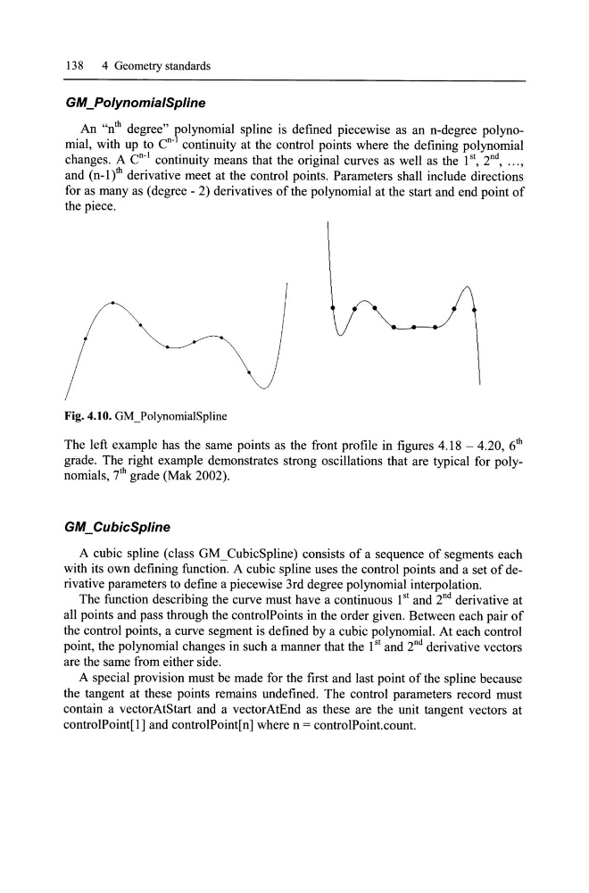
Fig. 4.10. GM]olynomialSpline
The left example has the same points as the front profile in figures 4.18 - 4.20, 6 th
grade. The right example demonstrates strong oscillations that are typical for polynomials, 7 th grade (Mak 2002).
GM_ CubicSpline
A cubic spline (class GM _ CubicSpline) consists of a sequence of segments each
with its own defining function. A cubic spline uses the control points and a set of derivative parameters to define a piecewise 3rd degree polynomial interpolation.
The function describing the curve must have a continuous 1 st and 2 nd derivative at
all points and pass through the controlPoints in the order given. Between each pair of
the control points, a curve segment is defined by a cubic polynomial. At each control
point, the polynomial changes in such a manner that the 1 st and 2 nd derivative vectors
are the same from either side.
A special provision must be made for the first and last point of the spline because
the tangent at these points remains undefined. The control parameters record must
contain a vectorAtStart and a vectorAtEnd as these are the unit tangent vectors at
controIPoint[l] and controIPoint[n] where n = controIPoint.count.
4 Geometry standards
GM_PolynomialSpline
An "n th degree" polynomial spline is defined piecewise as an n-degree polynomial, with up to C n - 1 continuity at the control points where the defining polynomial
changes. A C n - 1 continuity means that the original curves as well as the 1 st, 2 nd , ••• ,
and (n_l)th derivative meet at the control points. Parameters shall include directions
for as many as (degree - 2) derivatives ofthe polynomial at the start and end point of
the piece.
Fig. 4.10. GM]olynomialSpline
The left example has the same points as the front profile in figures 4.18 - 4.20, 6 th
grade. The right example demonstrates strong oscillations that are typical for polynomials, 7 th grade (Mak 2002).
GM_ CubicSpline
A cubic spline (class GM _ CubicSpline) consists of a sequence of segments each
with its own defining function. A cubic spline uses the control points and a set of derivative parameters to define a piecewise 3rd degree polynomial interpolation.
The function describing the curve must have a continuous 1 st and 2 nd derivative at
all points and pass through the controlPoints in the order given. Between each pair of
the control points, a curve segment is defined by a cubic polynomial. At each control
point, the polynomial changes in such a manner that the 1 st and 2 nd derivative vectors
are the same from either side.
A special provision must be made for the first and last point of the spline because
the tangent at these points remains undefined. The control parameters record must
contain a vectorAtStart and a vectorAtEnd as these are the unit tangent vectors at
controIPoint[l] and controIPoint[n] where n = controIPoint.count.