

58
Air Pollution and Turbulence: Modeling and Applications
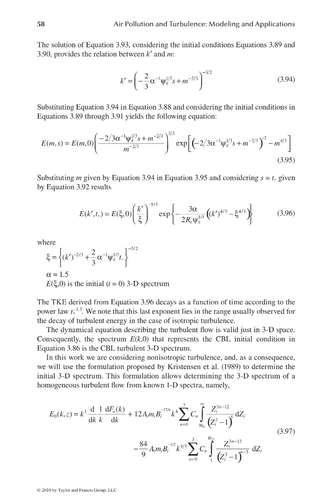
The solution of Equation 3.93, considering the initial conditions Equations 3.89 and
3.90, provides the relation between k′ and m:
−
−
−
ε
⎛
⎞
= − α ψ +
′ ⎜
⎟
⎝
⎠
3 2
1 13
2 3
2
3
k
s m
(3.94)
Substituting Equation 3.94 in Equation 3.88 and considering the initial conditions in
Equations 3.89 through 3.91 yields the following equation:
(
)
−
−
−
ε
−
−
ε
−
⎛
⎞
−
α ψ +
⎡
⎤
=
−α ψ+
−
⎜
⎟
⎢
⎥
⎣
⎦
⎝
⎠
5 3
1 13
2 3
2
1 13
2 3
4 3
2 3
2 3
( , )
( ,0)
exp
2 3
s m
E m s E m
s m
m
m
(3.95)
Substituting m given by Equation 3.94 in Equation 3.95 and considering s = t * given
by Equation 3.92 results
(
)
−
∗
ε
⎛ ⎞
⎧
⎫
α
′
= ξ
−
−ξ
′
′
⎨
⎬
⎜ ⎟
ξ
ψ
⎝ ⎠
⎩
⎭
5/3
4/3
4/3
1/3
3
( , )
( ,0)
exp
( )
2 e
k
E k t
E
k
R
(3.96)
where
−
−
−
ε ∗
⎧
⎫
ξ =
+ α ψ
′
⎨
⎬
⎩
⎭
3/2
2 /3
1 1/3
2
( )
3
k
t
α = 1.5
E(ξ,0) is the initial (t = 0) 3-D spectrum
The TKE derived from Equation 3.96 decays as a function of time according to the
power law
1.3
*
t
− . We note that this last exponent lies in the range usually observed for
the decay of turbulent energy in the case of isotropic turbulence.
The dynamical equation describing the turbulent fl ow is valid just in 3-D space.
Consequently, the spectrum E(k,0) that represents the CBL initial condition in
Equation 3.86 is the CBL turbulent 3-D spectrum.
In this work we are considering nonisotropic turbulence, and, as a consequence,
we will use the formulation proposed by Kristensen et al. (1989) to determine the
initial 3-D spectrum. This formulation allows determining the 3-D spectrum of a
homogeneous turbulent fl ow from known 1-D spectra, namely,
( )
( )
−
−
∞
−
=
−
−
=
=
+
−
−
−
∑ ∫
∑ ∫
17 6
1
2
3 2
3
3 12
3
4
0
5
3
0
3
3 12
4 3
5
3
0
1
d 1 d ( )
( , )
12
d
d
d
1
84
d
9
1
i
i
n
u
i
i i i
n
i
n
i
W
W
n
i
i i i
n
i
n
n
i
F k
Z
E k z k
Am B k
C
Z
k k
k
Z
Z
A m B k
C
Z
Z
(3.97)
© 2010 by Taylor and Francis Group, LLC
Air Pollution and Turbulence: Modeling and Applications
The solution of Equation 3.93, considering the initial conditions Equations 3.89 and
3.90, provides the relation between k′ and m:
−
−
−
ε
⎛
⎞
= − α ψ +
′ ⎜
⎟
⎝
⎠
3 2
1 13
2 3
2
3
k
s m
(3.94)
Substituting Equation 3.94 in Equation 3.88 and considering the initial conditions in
Equations 3.89 through 3.91 yields the following equation:
(
)
−
−
−
ε
−
−
ε
−
⎛
⎞
−
α ψ +
⎡
⎤
=
−α ψ+
−
⎜
⎟
⎢
⎥
⎣
⎦
⎝
⎠
5 3
1 13
2 3
2
1 13
2 3
4 3
2 3
2 3
( , )
( ,0)
exp
2 3
s m
E m s E m
s m
m
m
(3.95)
Substituting m given by Equation 3.94 in Equation 3.95 and considering s = t * given
by Equation 3.92 results
(
)
−
∗
ε
⎛ ⎞
⎧
⎫
α
′
= ξ
−
−ξ
′
′
⎨
⎬
⎜ ⎟
ξ
ψ
⎝ ⎠
⎩
⎭
5/3
4/3
4/3
1/3
3
( , )
( ,0)
exp
( )
2 e
k
E k t
E
k
R
(3.96)
where
−
−
−
ε ∗
⎧
⎫
ξ =
+ α ψ
′
⎨
⎬
⎩
⎭
3/2
2 /3
1 1/3
2
( )
3
k
t
α = 1.5
E(ξ,0) is the initial (t = 0) 3-D spectrum
The TKE derived from Equation 3.96 decays as a function of time according to the
power law
1.3
*
t
− . We note that this last exponent lies in the range usually observed for
the decay of turbulent energy in the case of isotropic turbulence.
The dynamical equation describing the turbulent fl ow is valid just in 3-D space.
Consequently, the spectrum E(k,0) that represents the CBL initial condition in
Equation 3.86 is the CBL turbulent 3-D spectrum.
In this work we are considering nonisotropic turbulence, and, as a consequence,
we will use the formulation proposed by Kristensen et al. (1989) to determine the
initial 3-D spectrum. This formulation allows determining the 3-D spectrum of a
homogeneous turbulent fl ow from known 1-D spectra, namely,
( )
( )
−
−
∞
−
=
−
−
=
=
+
−
−
−
∑ ∫
∑ ∫
17 6
1
2
3 2
3
3 12
3
4
0
5
3
0
3
3 12
4 3
5
3
0
1
d 1 d ( )
( , )
12
d
d
d
1
84
d
9
1
i
i
n
u
i
i i i
n
i
n
i
W
W
n
i
i i i
n
i
n
n
i
F k
Z
E k z k
Am B k
C
Z
k k
k
Z
Z
A m B k
C
Z
Z
(3.97)
© 2010 by Taylor and Francis Group, LLC