

52
Air Pollution and Turbulence: Modeling and Applications
Now defi ning n′ = bn, where =
*
1.5 / ( )
c
m i
b
z U f , Equations 3.70 through 3.72 can be
introduced into Equation 3.42 to obtain
( )
1 2
1 3
4 3
4 3
5 3
*
*
0
sin
d
0.09
( )
/
(1
)
i
i
c
i
m i
a n n
K
c
zz
b
w z
n
n
f
∞
α
ε
⎛
⎞
′
′
⎜
⎟
⎝
⎠
ψ
=
+ ′
′
⎡
⎤
⎢
⎥
⎣
⎦
∫
(3.73)
which expands to (Degrazia et al., 2001)
( )
( )
2 3
1 2 1 3
4 3
2 3
1 2 1 3
4 3
5 3
*
0
7.84
sin
d
( / )
0.09
(1
)
c
m
i
i
i
i
i
c
i
m i
c
f
X n n
z
z z
c
z
K
w z
n
n
f
∗
ε
∞
ε
α
∗
⎧
⎫
⎡
⎤
ψ
⎪
⎪
⎢
⎥
⎪
⎪
⎣
⎦
′
′
⎨
⎬
⎛ ⎞
⎪
⎪
ψ ⎜ ⎟
⎝ ⎠
⎪
⎪
⎩
⎭
=
+ ′
′
⎡
⎤
⎢
⎥
⎣
⎦
∫
(3.74)
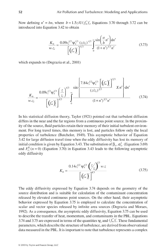
In his statistical diffusion theory, Taylor (1921) pointed out that turbulent diffusion
differs in the near and the far regions from a continuous point source. In the proximity of the source, fl uid particles retain their memory of their initial turbulent environment. For long travel times, this memory is lost, and particles follow only the local
properties of turbulence (Batchelor, 1949). This asymptotic behavior of Equation
3.42 for large diffusion travel time when the eddy diffusivity has lost its memory of
initial condition is given by Equation 3.43. The substitution of β ic , σ
2
ic (Equation 3.69)
and
=
E (
0)
i c
F n
(Equation 3.70) in Equation 3.43 leads to the following asymptotic
eddy diffusivity
( )
( )
ε
α
ψ
=
⎡
⎤
⎢
⎥
⎣
⎦
1 3
1 2
1 3
*
4 3
*
0.14 i
i
c
m i
z
c
w z
z
K
f
(3.75)
The eddy diffusivity expressed by Equation 3.74 depends on the geometry of the
source distribution and is suitable for calculation of the contaminant concentration
released by elevated continuous point sources. On the other hand, their asymptotic
behavior expressed by Equation 3.75 is employed to calculate the concentration of
scalar and vector species released by infi nite area sources (Degrazia and Moraes,
1992). As a consequence, the asymptotic eddy diffusivity, Equation 3.75 can be used
to describe the transfer of heat, momentum, and contaminants in the PBL. Equations
3.74 and 3.75 are expressed in terms of the quantities ψ ε and
*
( )
c
m i
f . These fundamental
parameters, which describe the structure of turbulence, are derived from observational
data measured in the PBL. It is important to note that turbulence represents a complex
© 2010 by Taylor and Francis Group, LLC
Air Pollution and Turbulence: Modeling and Applications
Now defi ning n′ = bn, where =
*
1.5 / ( )
c
m i
b
z U f , Equations 3.70 through 3.72 can be
introduced into Equation 3.42 to obtain
( )
1 2
1 3
4 3
4 3
5 3
*
*
0
sin
d
0.09
( )
/
(1
)
i
i
c
i
m i
a n n
K
c
zz
b
w z
n
n
f
∞
α
ε
⎛
⎞
′
′
⎜
⎟
⎝
⎠
ψ
=
+ ′
′
⎡
⎤
⎢
⎥
⎣
⎦
∫
(3.73)
which expands to (Degrazia et al., 2001)
( )
( )
2 3
1 2 1 3
4 3
2 3
1 2 1 3
4 3
5 3
*
0
7.84
sin
d
( / )
0.09
(1
)
c
m
i
i
i
i
i
c
i
m i
c
f
X n n
z
z z
c
z
K
w z
n
n
f
∗
ε
∞
ε
α
∗
⎧
⎫
⎡
⎤
ψ
⎪
⎪
⎢
⎥
⎪
⎪
⎣
⎦
′
′
⎨
⎬
⎛ ⎞
⎪
⎪
ψ ⎜ ⎟
⎝ ⎠
⎪
⎪
⎩
⎭
=
+ ′
′
⎡
⎤
⎢
⎥
⎣
⎦
∫
(3.74)
In his statistical diffusion theory, Taylor (1921) pointed out that turbulent diffusion
differs in the near and the far regions from a continuous point source. In the proximity of the source, fl uid particles retain their memory of their initial turbulent environment. For long travel times, this memory is lost, and particles follow only the local
properties of turbulence (Batchelor, 1949). This asymptotic behavior of Equation
3.42 for large diffusion travel time when the eddy diffusivity has lost its memory of
initial condition is given by Equation 3.43. The substitution of β ic , σ
2
ic (Equation 3.69)
and
=
E (
0)
i c
F n
(Equation 3.70) in Equation 3.43 leads to the following asymptotic
eddy diffusivity
( )
( )
ε
α
ψ
=
⎡
⎤
⎢
⎥
⎣
⎦
1 3
1 2
1 3
*
4 3
*
0.14 i
i
c
m i
z
c
w z
z
K
f
(3.75)
The eddy diffusivity expressed by Equation 3.74 depends on the geometry of the
source distribution and is suitable for calculation of the contaminant concentration
released by elevated continuous point sources. On the other hand, their asymptotic
behavior expressed by Equation 3.75 is employed to calculate the concentration of
scalar and vector species released by infi nite area sources (Degrazia and Moraes,
1992). As a consequence, the asymptotic eddy diffusivity, Equation 3.75 can be used
to describe the transfer of heat, momentum, and contaminants in the PBL. Equations
3.74 and 3.75 are expressed in terms of the quantities ψ ε and
*
( )
c
m i
f . These fundamental
parameters, which describe the structure of turbulence, are derived from observational
data measured in the PBL. It is important to note that turbulence represents a complex
© 2010 by Taylor and Francis Group, LLC