

Inversion of Atmospheric CO 2 Concentrations
289
In discussing the question of what has been learned from CO 2 inversions, we
adopt a number of principles identifi ed by Enting (2002):
Whatever cannot be modeled deterministically should be modeled
•
statistically.
Any statistical analysis is assuming (either explicitly or implicitly) some
•
statistical model. Clearly, explicit identifi cation of the assumptions is
preferable.
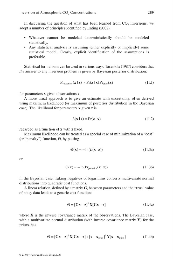
Statistical formalisms can be used in various ways. Tarantola (1987) considers that
the answer to any inversion problem is given by Bayesian posterior distribution:
posterior
prior
Pr
( | ) Pr( | ) Pr ( )
∝
x z
z x
x
(11.1)
for parameters x given observations z.
A more usual approach is to give an estimate with uncertainty, often derived
using maximum likelihood (or maximum of posterior distribution in the Bayesian
case). The likelihood for parameters x given z is
( | ) Pr( | )
L
=
x z
z x
(11.2)
regarded as a function of x with z fi xed.
Maximum likelihood can be treated as a special case of minimization of a “cost”
(or “penalty”) function, Θ, by putting
( )
ln( ( | ))
L
Θ = −
x
x z
(11.3a)
or
posterior
( )
ln(Pr
( | ))
Θ = −
x
xz
(11.3b)
in the Bayesian case. Taking negatives of logarithms converts multivariate normal
distributions into quadratic cost functions.
A linear relation, defi ned by a matrix G, between parameters and the “true” value
of noisy data leads to a generic cost function:
T
[
] [
]
Θ =
−
−
Gx z X Gx z
(11.4a)
where X is the inverse covariance matrix of the observations. The Bayesian case,
with a multivariate normal distribution (with inverse covariance matrix Y) for the
priors, has
T
T
prior
prior
[
] [
] [
] [
]
Θ =
−
− + −
−
Gx z X Gx z
x x
Y x x
(11.4b)
© 2010 by Taylor and Francis Group, LLC
289
In discussing the question of what has been learned from CO 2 inversions, we
adopt a number of principles identifi ed by Enting (2002):
Whatever cannot be modeled deterministically should be modeled
•
statistically.
Any statistical analysis is assuming (either explicitly or implicitly) some
•
statistical model. Clearly, explicit identifi cation of the assumptions is
preferable.
Statistical formalisms can be used in various ways. Tarantola (1987) considers that
the answer to any inversion problem is given by Bayesian posterior distribution:
posterior
prior
Pr
( | ) Pr( | ) Pr ( )
∝
x z
z x
x
(11.1)
for parameters x given observations z.
A more usual approach is to give an estimate with uncertainty, often derived
using maximum likelihood (or maximum of posterior distribution in the Bayesian
case). The likelihood for parameters x given z is
( | ) Pr( | )
L
=
x z
z x
(11.2)
regarded as a function of x with z fi xed.
Maximum likelihood can be treated as a special case of minimization of a “cost”
(or “penalty”) function, Θ, by putting
( )
ln( ( | ))
L
Θ = −
x
x z
(11.3a)
or
posterior
( )
ln(Pr
( | ))
Θ = −
x
xz
(11.3b)
in the Bayesian case. Taking negatives of logarithms converts multivariate normal
distributions into quadratic cost functions.
A linear relation, defi ned by a matrix G, between parameters and the “true” value
of noisy data leads to a generic cost function:
T
[
] [
]
Θ =
−
−
Gx z X Gx z
(11.4a)
where X is the inverse covariance matrix of the observations. The Bayesian case,
with a multivariate normal distribution (with inverse covariance matrix Y) for the
priors, has
T
T
prior
prior
[
] [
] [
] [
]
Θ =
−
− + −
−
Gx z X Gx z
x x
Y x x
(11.4b)
© 2010 by Taylor and Francis Group, LLC