

Atmospheric Dispersion with a Large-Eddy Simulation
249
horizontal direction and 1 km in the vertical direction, with a resolution of 96 grid
points in each of the three directions.
Simulations started from a laminar fl ow, with the geostrophic wind constant
throughout the numerical domain. In order to have a strong capping inversion above
the simulated PBL, the initial mean virtual potential temperature profi le was 300 K
below an initial PBL height, (z i ) 0 , that increases by a total of 8 K across six Δz levels
and increases with a lapse rate of 3 K/km above that. External parameters like the
extent of the domain, the grid size, the geostrophic winds, the surface heat fl ux, and
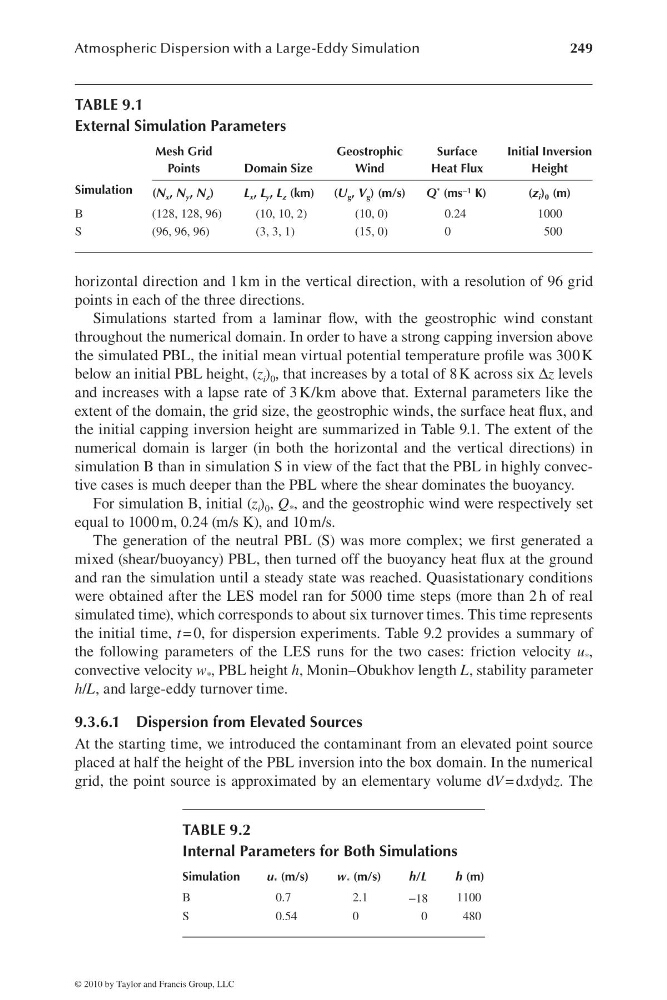
the initial capping inversion height are summarized in Table 9.1. The extent of the
numerical domain is larger (in both the horizontal and the vertical directions) in
simulation B than in simulation S in view of the fact that the PBL in highly convective cases is much deeper than the PBL where the shear dominates the buoyancy.
For simulation B, initial (z i ) 0 , Q * , and the geostrophic wind were respectively set
equal to 1000 m, 0.24 (m/s K), and 10 m/s.
The generation of the neutral PBL (S) was more complex; we fi rst generated a
mixed (shear/buoyancy) PBL, then turned off the buoyancy heat fl ux at the ground
and ran the simulation until a steady state was reached. Quasistationary conditions
were obtained after the LES model ran for 5000 time steps (more than 2 h of real
simulated time), which corresponds to about six turnover times. This time represents
the initial time, t = 0, for dispersion experiments. Table 9.2 provides a summary of
the following parameters of the LES runs for the two cases: friction velocity u * ,
convective velocity w * , PBL height h, Monin–Obukhov length L, stability parameter
h/L, and large-eddy turnover time.
9.3.6.1 Dispersion from Elevated Sources
At the starting time, we introduced the contaminant from an elevated point source
placed at half the height of the PBL inversion into the box domain. In the numerical
grid, the point source is approximated by an elementary volume dV = dxdydz. The
TABLE 9.1
External Simulation Parameters
Mesh Grid
Points
Domain Size
Geostrophic
Wind
Surface
Heat Flux
Initial Inversion
Height
Simulation
(N x , N y , N z )
L x , L y , L z (km)
(U g , V g ) (m/s)
Q * (ms −1 K)
(z i ) 0 (m)
B
(128, 128, 96)
(10, 10, 2)
(10, 0)
0.24
1000
S
(96, 96, 96)
(3, 3, 1)
(15, 0)
0
500
TABLE 9.2
Internal Parameters for Both Simulations
Simulation
u * (m/s)
w * (m/s)
h/L
h (m)
B
0.7
2.1
−18
1100
S
0.54
0
0
480
© 2010 by Taylor and Francis Group, LLC
249
horizontal direction and 1 km in the vertical direction, with a resolution of 96 grid
points in each of the three directions.
Simulations started from a laminar fl ow, with the geostrophic wind constant
throughout the numerical domain. In order to have a strong capping inversion above
the simulated PBL, the initial mean virtual potential temperature profi le was 300 K
below an initial PBL height, (z i ) 0 , that increases by a total of 8 K across six Δz levels
and increases with a lapse rate of 3 K/km above that. External parameters like the
extent of the domain, the grid size, the geostrophic winds, the surface heat fl ux, and
the initial capping inversion height are summarized in Table 9.1. The extent of the
numerical domain is larger (in both the horizontal and the vertical directions) in
simulation B than in simulation S in view of the fact that the PBL in highly convective cases is much deeper than the PBL where the shear dominates the buoyancy.
For simulation B, initial (z i ) 0 , Q * , and the geostrophic wind were respectively set
equal to 1000 m, 0.24 (m/s K), and 10 m/s.
The generation of the neutral PBL (S) was more complex; we fi rst generated a
mixed (shear/buoyancy) PBL, then turned off the buoyancy heat fl ux at the ground
and ran the simulation until a steady state was reached. Quasistationary conditions
were obtained after the LES model ran for 5000 time steps (more than 2 h of real
simulated time), which corresponds to about six turnover times. This time represents
the initial time, t = 0, for dispersion experiments. Table 9.2 provides a summary of
the following parameters of the LES runs for the two cases: friction velocity u * ,
convective velocity w * , PBL height h, Monin–Obukhov length L, stability parameter
h/L, and large-eddy turnover time.
9.3.6.1 Dispersion from Elevated Sources
At the starting time, we introduced the contaminant from an elevated point source
placed at half the height of the PBL inversion into the box domain. In the numerical
grid, the point source is approximated by an elementary volume dV = dxdydz. The
TABLE 9.1
External Simulation Parameters
Mesh Grid
Points
Domain Size
Geostrophic
Wind
Surface
Heat Flux
Initial Inversion
Height
Simulation
(N x , N y , N z )
L x , L y , L z (km)
(U g , V g ) (m/s)
Q * (ms −1 K)
(z i ) 0 (m)
B
(128, 128, 96)
(10, 10, 2)
(10, 0)
0.24
1000
S
(96, 96, 96)
(3, 3, 1)
(15, 0)
0
500
TABLE 9.2
Internal Parameters for Both Simulations
Simulation
u * (m/s)
w * (m/s)
h/L
h (m)
B
0.7
2.1
−18
1100
S
0.54
0
0
480
© 2010 by Taylor and Francis Group, LLC