

230
Air Pollution and Turbulence: Modeling and Applications
the ground-level concentrations measured at a network of ground-level samplers,
following the procedure reported in Equations 8.41and 8.42. The inverse procedure
was applied to data from the real fi eld (the Copenhagen tracer experiment, performed
on October 19, 1978), where some level of noise in the data is expected. Roberti
et al. (2007) made use of the second-order Tikhonov regularization and determined
the regularization parameter according to the L-curve scheme (Hansen, 1992).
In the Copenhagen experiment, 39 ground-level samplers were located in three
crosswind arcs, located at 2–6 km from the releasing point, and the main meteorological parameters were measured at three heights (10, 120, and 200 m) along a tower
and the emission was released from the same tower at 115 m.
The Lagrangian particle model LAMBDA, that is, the SPRAY version for fl at
terrain, was used to simulate the direct (or forward) problem, while the inverse problem was formulated as an optimization problem.
The time period for the experiment and, consequently, of the emission rate
estimation was 50 min. The emission rate was assumed variable with time but it
was constant and equal to 3.2 g s −1 in the experiment. Thus, in the simulation, the
unknown source term could be represented by the vector: Q = [Q 1 , Q 2 , Q 3 , Q 4 , Q 5 ] T ,
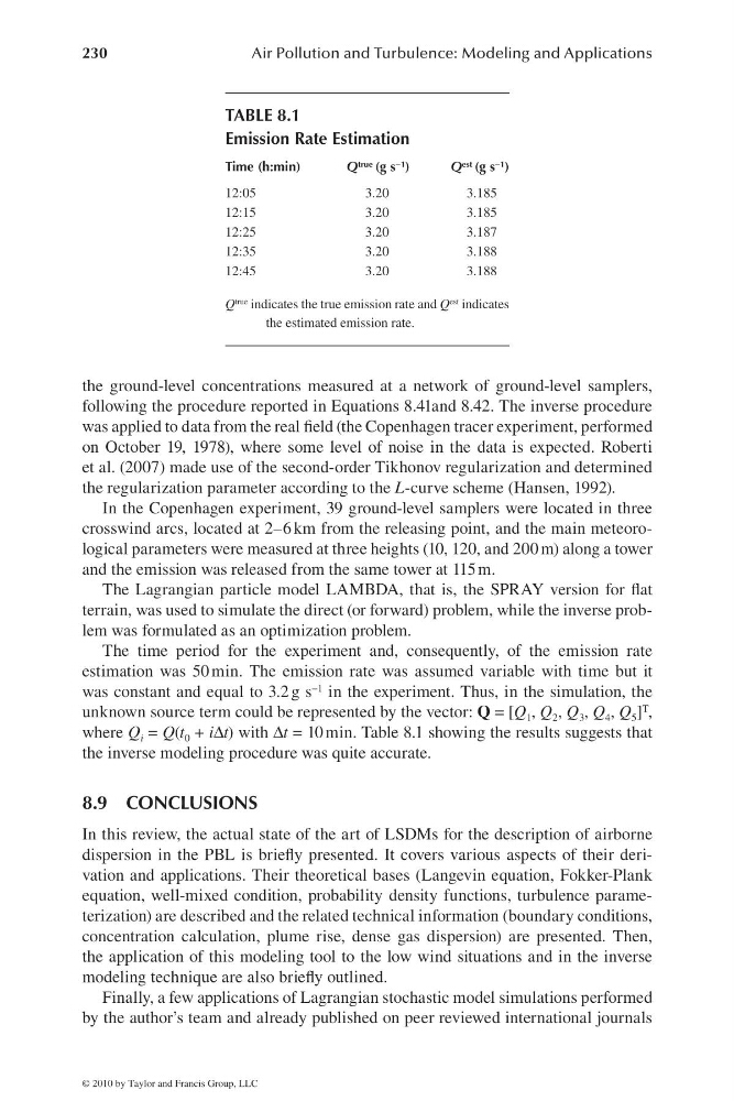
where Q i = Q(t 0 + iΔt) with Δt = 10 min. Table 8.1 showing the results suggests that
the inverse modeling procedure was quite accurate.
8.9 CONCLUSIONS
In this review, the actual state of the art of LSDMs for the description of airborne
dispersion in the PBL is briefl y presented. It covers various aspects of their derivation and applications. Their theoretical bases (Langevin equation, Fokker-Plank
equation, well-mixed condition, probability density functions, turbulence parameterization) are described and the related technical information (boundary conditions,
concentration calculation, plume rise, dense gas dispersion) are presented. Then,
the application of this modeling tool to the low wind situations and in the inverse
modeling technique are also briefl y outlined.
Finally, a few applications of Lagrangian stochastic model simulations performed
by the author’s team and already published on peer reviewed international journals
TABLE 8.1
Emission Rate Estimation
Time (h:min)
Q true (g s −1 )
Q est (g s −1 )
12:05
3.20
3.185
12:15
3.20
3.185
12:25
3.20
3.187
12:35
3.20
3.188
12:45
3.20
3.188
Q true indicates the true emission rate and Q est indicates
the estimated emission rate.
© 2010 by Taylor and Francis Group, LLC
Air Pollution and Turbulence: Modeling and Applications
the ground-level concentrations measured at a network of ground-level samplers,
following the procedure reported in Equations 8.41and 8.42. The inverse procedure
was applied to data from the real fi eld (the Copenhagen tracer experiment, performed
on October 19, 1978), where some level of noise in the data is expected. Roberti
et al. (2007) made use of the second-order Tikhonov regularization and determined
the regularization parameter according to the L-curve scheme (Hansen, 1992).
In the Copenhagen experiment, 39 ground-level samplers were located in three
crosswind arcs, located at 2–6 km from the releasing point, and the main meteorological parameters were measured at three heights (10, 120, and 200 m) along a tower
and the emission was released from the same tower at 115 m.
The Lagrangian particle model LAMBDA, that is, the SPRAY version for fl at
terrain, was used to simulate the direct (or forward) problem, while the inverse problem was formulated as an optimization problem.
The time period for the experiment and, consequently, of the emission rate
estimation was 50 min. The emission rate was assumed variable with time but it
was constant and equal to 3.2 g s −1 in the experiment. Thus, in the simulation, the
unknown source term could be represented by the vector: Q = [Q 1 , Q 2 , Q 3 , Q 4 , Q 5 ] T ,
where Q i = Q(t 0 + iΔt) with Δt = 10 min. Table 8.1 showing the results suggests that
the inverse modeling procedure was quite accurate.
8.9 CONCLUSIONS
In this review, the actual state of the art of LSDMs for the description of airborne
dispersion in the PBL is briefl y presented. It covers various aspects of their derivation and applications. Their theoretical bases (Langevin equation, Fokker-Plank
equation, well-mixed condition, probability density functions, turbulence parameterization) are described and the related technical information (boundary conditions,
concentration calculation, plume rise, dense gas dispersion) are presented. Then,
the application of this modeling tool to the low wind situations and in the inverse
modeling technique are also briefl y outlined.
Finally, a few applications of Lagrangian stochastic model simulations performed
by the author’s team and already published on peer reviewed international journals
TABLE 8.1
Emission Rate Estimation
Time (h:min)
Q true (g s −1 )
Q est (g s −1 )
12:05
3.20
3.185
12:15
3.20
3.185
12:25
3.20
3.187
12:35
3.20
3.188
12:45
3.20
3.188
Q true indicates the true emission rate and Q est indicates
the estimated emission rate.
© 2010 by Taylor and Francis Group, LLC