

228
Air Pollution and Turbulence: Modeling and Applications
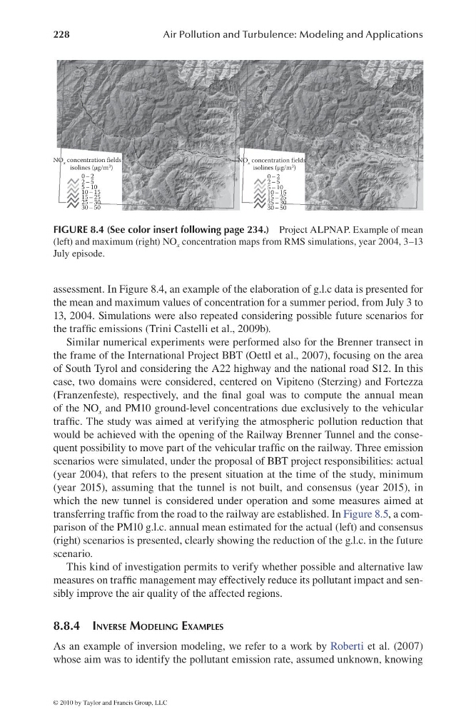
assessment. In Figure 8.4, an example of the elaboration of g.l.c data is presented for
the mean and maximum values of concentration for a summer period, from July 3 to
13, 2004. Simulations were also repeated considering possible future scenarios for
the traffi c emissions (Trini Castelli et al., 2009b).
Similar numerical experiments were performed also for the Brenner transect in
the frame of the International Project BBT (Oettl et al., 2007), focusing on the area
of South Tyrol and considering the A22 highway and the national road S12. In this
case, two domains were considered, centered on Vipiteno (Sterzing) and Fortezza
(Franzenfeste), respectively, and the fi nal goal was to compute the annual mean
of the NO x and PM10 ground-level concentrations due exclusively to the vehicular
traffi c. The study was aimed at verifying the atmospheric pollution reduction that
would be achieved with the opening of the Railway Brenner Tunnel and the consequent possibility to move part of the vehicular traffi c on the railway. Three emission
scenarios were simulated, under the proposal of BBT project responsibilities: actual
(year 2004), that refers to the present situation at the time of the study, minimum
(year 2015), assuming that the tunnel is not built, and consensus (year 2015), in
which the new tunnel is considered under operation and some measures aimed at
transferring traffi c from the road to the railway are established. In Figure 8.5, a comparison of the PM10 g.l.c. annual mean estimated for the actual (left) and consensus
(right) scenarios is presented, clearly showing the reduction of the g.l.c. in the future
scenario.
This kind of investigation permits to verify whether possible and alternative law
measures on traffi c management may effectively reduce its pollutant impact and sensibly improve the air quality of the affected regions.
8.8.4 INVERSE MODELING EXAMPLES
As an example of inversion modeling, we refer to a work by Roberti et al. (2007)
whose aim was to identify the pollutant emission rate, assumed unknown, knowing
0 – 2
2 – 5
5 – 10
10 – 15
15 – 25
25 – 30
30 – 50
NO x concentration fields
0 – 2
2 – 5
5 – 10
10 – 15
15 – 25
25 – 30
30 – 50
NO x concentration fields
isolines (μg/m 3 )
isolines (μg/m 3 )
FIGURE 8.4 (See color insert following page 234.) Project ALPNAP. Example of mean
(left) and maximum (right) NO x concentration maps from RMS simulations, year 2004, 3–13
July episode.
© 2010 by Taylor and Francis Group, LLC
Air Pollution and Turbulence: Modeling and Applications
assessment. In Figure 8.4, an example of the elaboration of g.l.c data is presented for
the mean and maximum values of concentration for a summer period, from July 3 to
13, 2004. Simulations were also repeated considering possible future scenarios for
the traffi c emissions (Trini Castelli et al., 2009b).
Similar numerical experiments were performed also for the Brenner transect in
the frame of the International Project BBT (Oettl et al., 2007), focusing on the area
of South Tyrol and considering the A22 highway and the national road S12. In this
case, two domains were considered, centered on Vipiteno (Sterzing) and Fortezza
(Franzenfeste), respectively, and the fi nal goal was to compute the annual mean
of the NO x and PM10 ground-level concentrations due exclusively to the vehicular
traffi c. The study was aimed at verifying the atmospheric pollution reduction that
would be achieved with the opening of the Railway Brenner Tunnel and the consequent possibility to move part of the vehicular traffi c on the railway. Three emission
scenarios were simulated, under the proposal of BBT project responsibilities: actual
(year 2004), that refers to the present situation at the time of the study, minimum
(year 2015), assuming that the tunnel is not built, and consensus (year 2015), in
which the new tunnel is considered under operation and some measures aimed at
transferring traffi c from the road to the railway are established. In Figure 8.5, a comparison of the PM10 g.l.c. annual mean estimated for the actual (left) and consensus
(right) scenarios is presented, clearly showing the reduction of the g.l.c. in the future
scenario.
This kind of investigation permits to verify whether possible and alternative law
measures on traffi c management may effectively reduce its pollutant impact and sensibly improve the air quality of the affected regions.
8.8.4 INVERSE MODELING EXAMPLES
As an example of inversion modeling, we refer to a work by Roberti et al. (2007)
whose aim was to identify the pollutant emission rate, assumed unknown, knowing
0 – 2
2 – 5
5 – 10
10 – 15
15 – 25
25 – 30
30 – 50
NO x concentration fields
0 – 2
2 – 5
5 – 10
10 – 15
15 – 25
25 – 30
30 – 50
NO x concentration fields
isolines (μg/m 3 )
isolines (μg/m 3 )
FIGURE 8.4 (See color insert following page 234.) Project ALPNAP. Example of mean
(left) and maximum (right) NO x concentration maps from RMS simulations, year 2004, 3–13
July episode.
© 2010 by Taylor and Francis Group, LLC