

Pollutant Dispersion Simulation in the ABL by the GILTT Method
197
the statistical index FA5 (fraction of data [%, normalized to 1] for 0.2 ≤ (C p /C o ) ≤ 5),
usually for simulations and complex terrain. Best results are obtained when FA5
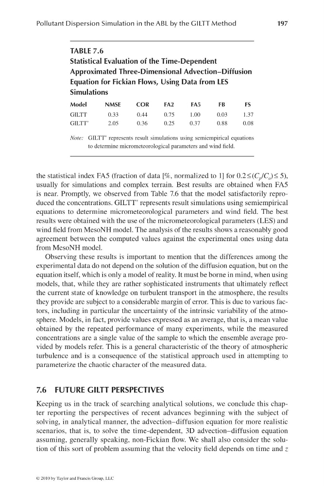
is near. Promptly, we observed from Table 7.6 that the model satisfactorily reproduced the concentrations. GILTT * represents result simulations using semiempirical
equations to determine micrometeorological parameters and wind fi eld. The best
results were obtained with the use of the micrometeorological parameters (LES) and
wind fi eld from MesoNH model. The analysis of the results shows a reasonably good
agreement between the computed values against the experimental ones using data
from MesoNH model.
Observing these results is important to mention that the differences among the
experimental data do not depend on the solution of the diffusion equation, but on the
equation itself, which is only a model of reality. It must be borne in mind, when using
models, that, while they are rather sophisticated instruments that ultimately refl ect
the current state of knowledge on turbulent transport in the atmosphere, the results
they provide are subject to a considerable margin of error. This is due to various factors, including in particular the uncertainty of the intrinsic variability of the atmosphere. Models, in fact, provide values expressed as an average, that is, a mean value
obtained by the repeated performance of many experiments, while the measured
concentrations are a single value of the sample to which the ensemble average provided by models refer. This is a general characteristic of the theory of atmospheric
turbulence and is a consequence of the statistical approach used in attempting to
parameterize the chaotic character of the measured data.
7.6 FUTURE GILTT PERSPECTIVES
Keeping us in the track of searching analytical solutions, we conclude this chapter reporting the perspectives of recent advances beginning with the subject of
solving, in analytical manner, the advection–diffusion equation for more realistic
scenarios, that is, to solve the time-dependent, 3D advection–diffusion equation
assuming, generally speaking, non-Fickian fl ow. We shall also consider the solution of this sort of problem assuming that the velocity fi eld depends on time and z
TABLE 7.6
Statistical Evaluation of the Time-Dependent
Approximated Three-Dimensional Advection–Diffusion
Equation for Fickian Flows, Using Data from LES
Simulations
Model
NMSE
COR
FA2
FA5
FB
FS
GILTT
0.33
0.44
0.75
1.00
0.03
1.37
GILTT *
2.05
0.36
0.25
0.37
0.88
0.08
Note: GILTT * represents result simulations using semiempirical equations
to determine micrometeorological parameters and wind fi eld.
© 2010 by Taylor and Francis Group, LLC
197
the statistical index FA5 (fraction of data [%, normalized to 1] for 0.2 ≤ (C p /C o ) ≤ 5),
usually for simulations and complex terrain. Best results are obtained when FA5
is near. Promptly, we observed from Table 7.6 that the model satisfactorily reproduced the concentrations. GILTT * represents result simulations using semiempirical
equations to determine micrometeorological parameters and wind fi eld. The best
results were obtained with the use of the micrometeorological parameters (LES) and
wind fi eld from MesoNH model. The analysis of the results shows a reasonably good
agreement between the computed values against the experimental ones using data
from MesoNH model.
Observing these results is important to mention that the differences among the
experimental data do not depend on the solution of the diffusion equation, but on the
equation itself, which is only a model of reality. It must be borne in mind, when using
models, that, while they are rather sophisticated instruments that ultimately refl ect
the current state of knowledge on turbulent transport in the atmosphere, the results
they provide are subject to a considerable margin of error. This is due to various factors, including in particular the uncertainty of the intrinsic variability of the atmosphere. Models, in fact, provide values expressed as an average, that is, a mean value
obtained by the repeated performance of many experiments, while the measured
concentrations are a single value of the sample to which the ensemble average provided by models refer. This is a general characteristic of the theory of atmospheric
turbulence and is a consequence of the statistical approach used in attempting to
parameterize the chaotic character of the measured data.
7.6 FUTURE GILTT PERSPECTIVES
Keeping us in the track of searching analytical solutions, we conclude this chapter reporting the perspectives of recent advances beginning with the subject of
solving, in analytical manner, the advection–diffusion equation for more realistic
scenarios, that is, to solve the time-dependent, 3D advection–diffusion equation
assuming, generally speaking, non-Fickian fl ow. We shall also consider the solution of this sort of problem assuming that the velocity fi eld depends on time and z
TABLE 7.6
Statistical Evaluation of the Time-Dependent
Approximated Three-Dimensional Advection–Diffusion
Equation for Fickian Flows, Using Data from LES
Simulations
Model
NMSE
COR
FA2
FA5
FB
FS
GILTT
0.33
0.44
0.75
1.00
0.03
1.37
GILTT *
2.05
0.36
0.25
0.37
0.88
0.08
Note: GILTT * represents result simulations using semiempirical equations
to determine micrometeorological parameters and wind fi eld.
© 2010 by Taylor and Francis Group, LLC