

Pollutant Dispersion Simulation in the ABL by the GILTT Method
189
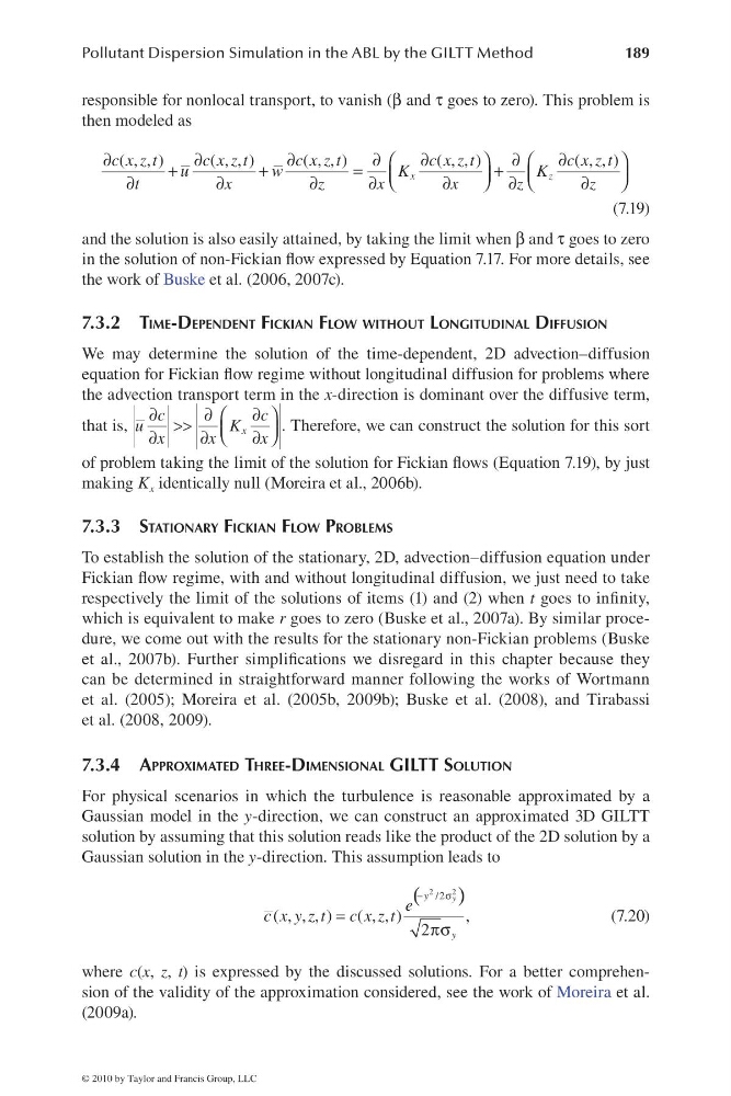
responsible for nonlocal transport, to vanish (β and τ goes to zero). This problem is
then modeled as
∂
∂
∂
∂
∂
∂
∂
⎛
⎞
⎛
⎞
+
+
=
+
⎜
⎟
⎜
⎟
⎝
⎠
⎝
⎠
∂
∂
∂
∂
∂
∂
∂
( , , )
( , , )
( , , )
( , , )
( , , )
x
z
c x z t
c x z t
c x z t
c x z t
c x z t
u
w
K
K
t
x
z
x
x
z
z
(7.19)
and the solution is also easily attained, by taking the limit when β and τ goes to zero
in the solution of non-Fickian fl ow expressed by Equation 7.17. For more details, see
the work of Buske et al. (2006, 2007c).
7.3.2 TIME-DEPENDENT FICKIAN FLOW WITHOUT LONGITUDINAL DIFFUSION
We may determine the solution of the time-dependent, 2D advection–diffusion
equation for Fickian fl ow regime without longitudinal diffusion for problems where
the advection transport term in the x-direction is dominant over the diffusive term,
that is,
∂
∂
∂
⎛
⎞
>>
⎜
⎟
⎝
⎠
∂
∂
∂
x
c
c
u
K
x
x
x
. Therefore, we can construct the solution for this sort
of problem taking the limit of the solution for Fickian fl ows (Equation 7.19), by just
making K x identically null (Moreira et al., 2006b).
7.3.3 STATIONARY FICKIAN FLOW PROBLEMS
To establish the solution of the stationary, 2D, advection–diffusion equation under
Fickian fl ow regime, with and without longitudinal diffusion, we just need to take
respectively the limit of the solutions of items (1) and (2) when t goes to infi nity,
which is equivalent to make r goes to zero (Buske et al., 2007a). By similar procedure, we come out with the results for the stationary non-Fickian problems (Buske
et al., 2007b). Further simplifi cations we disregard in this chapter because they
can be determined in straightforward manner following the works of Wortmann
et al. (2005); Moreira et al. (2005b, 2009b); Buske et al. (2008), and Tirabassi
et al. (2008, 2009).
7.3.4 APPROXIMATED THREE-DIMENSIONAL GILTT SOLUTION
For physical scenarios in which the turbulence is reasonable approximated by a
Gaussian model in the y-direction, we can construct an approximated 3D GILTT
solution by assuming that this solution reads like the product of the 2D solution by a
Gaussian solution in the y-direction. This assumption leads to
(
)
−
σ
=
πσ
2
2
/2
( , , , ) ( , , )
,
2
y
y
y
e
c x y z t c x z t
(7.20)
where c(x, z, t) is expressed by the discussed solutions. For a better comprehension of the validity of the approximation considered, see the work of Moreira et al.
(2009a).
© 2010 by Taylor and Francis Group, LLC
189
responsible for nonlocal transport, to vanish (β and τ goes to zero). This problem is
then modeled as
∂
∂
∂
∂
∂
∂
∂
⎛
⎞
⎛
⎞
+
+
=
+
⎜
⎟
⎜
⎟
⎝
⎠
⎝
⎠
∂
∂
∂
∂
∂
∂
∂
( , , )
( , , )
( , , )
( , , )
( , , )
x
z
c x z t
c x z t
c x z t
c x z t
c x z t
u
w
K
K
t
x
z
x
x
z
z
(7.19)
and the solution is also easily attained, by taking the limit when β and τ goes to zero
in the solution of non-Fickian fl ow expressed by Equation 7.17. For more details, see
the work of Buske et al. (2006, 2007c).
7.3.2 TIME-DEPENDENT FICKIAN FLOW WITHOUT LONGITUDINAL DIFFUSION
We may determine the solution of the time-dependent, 2D advection–diffusion
equation for Fickian fl ow regime without longitudinal diffusion for problems where
the advection transport term in the x-direction is dominant over the diffusive term,
that is,
∂
∂
∂
⎛
⎞
>>
⎜
⎟
⎝
⎠
∂
∂
∂
x
c
c
u
K
x
x
x
. Therefore, we can construct the solution for this sort
of problem taking the limit of the solution for Fickian fl ows (Equation 7.19), by just
making K x identically null (Moreira et al., 2006b).
7.3.3 STATIONARY FICKIAN FLOW PROBLEMS
To establish the solution of the stationary, 2D, advection–diffusion equation under
Fickian fl ow regime, with and without longitudinal diffusion, we just need to take
respectively the limit of the solutions of items (1) and (2) when t goes to infi nity,
which is equivalent to make r goes to zero (Buske et al., 2007a). By similar procedure, we come out with the results for the stationary non-Fickian problems (Buske
et al., 2007b). Further simplifi cations we disregard in this chapter because they
can be determined in straightforward manner following the works of Wortmann
et al. (2005); Moreira et al. (2005b, 2009b); Buske et al. (2008), and Tirabassi
et al. (2008, 2009).
7.3.4 APPROXIMATED THREE-DIMENSIONAL GILTT SOLUTION
For physical scenarios in which the turbulence is reasonable approximated by a
Gaussian model in the y-direction, we can construct an approximated 3D GILTT
solution by assuming that this solution reads like the product of the 2D solution by a
Gaussian solution in the y-direction. This assumption leads to
(
)
−
σ
=
πσ
2
2
/2
( , , , ) ( , , )
,
2
y
y
y
e
c x y z t c x z t
(7.20)
where c(x, z, t) is expressed by the discussed solutions. For a better comprehension of the validity of the approximation considered, see the work of Moreira et al.
(2009a).
© 2010 by Taylor and Francis Group, LLC