

Pollutant Dispersion Simulation in the ABL by the GILTT Method
187
and B 3 (x) by taking average values for the eddy diffusivity and its derivative in the
x variable. Here it is important to mention that no approximation is made on the
derivatives appearing in the advection–diffusion equation. From this procedure, it
turns out that problem 7.11 simplifi es to a set of ordinary differential equations, in
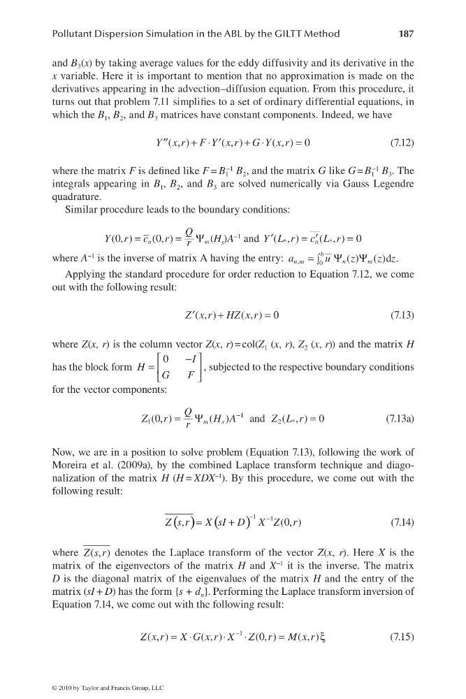
which the B 1 , B 2 , and B 3 matrices have constant components. Indeed, we have
( , )
( , )
( , ) 0
Y x r F Y x r G Y x r
+ ⋅
+ ⋅
=
′′
′
(7.12)
where the matrix F is defi ned like F = B 1
−1 B 2 , and the matrix G like G = B 1
−1 B 3 . The
integrals appearing in B 1 , B 2 , and B 3 are solved numerically via Gauss Legendre
quadrature.
Similar procedure leads to the boundary conditions:
=
= Ψ
(0, )
(0, )
n
m
Q
Y r c
r
r
(H s )A −1 and
*
*
( , )
( , ) 0
n
Y L r c L r
=
=
′
′
where A −1 is the inverse of matrix A having the entry:
=
Ψ
Ψ
∫⎯
,
0
( ) ( )d .
h
n m
n
m
a
u
z
z z
Applying the standard procedure for order reduction to Equation 7.12, we come
out with the following result:
+
=
′( , )
( , ) 0
Z x r HZ x r
(7.13)
where Z(x, r) is the column vector Z(x, r) = col(Z 1 (x, r), Z 2 (x, r)) and the matrix H
has the block form
0
I
H
G
F
−
⎡
⎤
= ⎢
⎥
⎣
⎦
, subjected to the respective boundary conditions
for the vector components:
−
= Ψ
=
1
1
2
*
(0, )
( )
and
( , ) 0
m
s
Q
Z r
H A
Z L r
r
(7.13a)
Now, we are in a position to solve problem (Equation 7.13), following the work of
Moreira et al. (2009a), by the combined Laplace transform technique and diagonalization of the matrix H (H = XDX −1 ). By this procedure, we come out with the
following result:
( ) (
)
1
1
,
( 0 , )
Z s r
X sI D X Z r
−
−
=
+
(7.14)
where ( , )
Z s r denotes the Laplace transform of the vector Z(x, r). Here X is the
matrix of the eigenvectors of the matrix H and X −1 it is the inverse. The matrix
D is the diagonal matrix of the eigenvalues of the matrix H and the entry of the
matrix (sI + D) has the form {s + d n }. Performing the Laplace transform inversion of
Equation 7.14, we come out with the following result:
1
( , )
( , )
(0, )
( , )
Z x r
X G x r X Z r M x r
−
= ⋅
⋅
⋅
=
ξ
(7.15)
© 2010 by Taylor and Francis Group, LLC
187
and B 3 (x) by taking average values for the eddy diffusivity and its derivative in the
x variable. Here it is important to mention that no approximation is made on the
derivatives appearing in the advection–diffusion equation. From this procedure, it
turns out that problem 7.11 simplifi es to a set of ordinary differential equations, in
which the B 1 , B 2 , and B 3 matrices have constant components. Indeed, we have
( , )
( , )
( , ) 0
Y x r F Y x r G Y x r
+ ⋅
+ ⋅
=
′′
′
(7.12)
where the matrix F is defi ned like F = B 1
−1 B 2 , and the matrix G like G = B 1
−1 B 3 . The
integrals appearing in B 1 , B 2 , and B 3 are solved numerically via Gauss Legendre
quadrature.
Similar procedure leads to the boundary conditions:
=
= Ψ
(0, )
(0, )
n
m
Q
Y r c
r
r
(H s )A −1 and
*
*
( , )
( , ) 0
n
Y L r c L r
=
=
′
′
where A −1 is the inverse of matrix A having the entry:
=
Ψ
Ψ
∫⎯
,
0
( ) ( )d .
h
n m
n
m
a
u
z
z z
Applying the standard procedure for order reduction to Equation 7.12, we come
out with the following result:
+
=
′( , )
( , ) 0
Z x r HZ x r
(7.13)
where Z(x, r) is the column vector Z(x, r) = col(Z 1 (x, r), Z 2 (x, r)) and the matrix H
has the block form
0
I
H
G
F
−
⎡
⎤
= ⎢
⎥
⎣
⎦
, subjected to the respective boundary conditions
for the vector components:
−
= Ψ
=
1
1
2
*
(0, )
( )
and
( , ) 0
m
s
Q
Z r
H A
Z L r
r
(7.13a)
Now, we are in a position to solve problem (Equation 7.13), following the work of
Moreira et al. (2009a), by the combined Laplace transform technique and diagonalization of the matrix H (H = XDX −1 ). By this procedure, we come out with the
following result:
( ) (
)
1
1
,
( 0 , )
Z s r
X sI D X Z r
−
−
=
+
(7.14)
where ( , )
Z s r denotes the Laplace transform of the vector Z(x, r). Here X is the
matrix of the eigenvectors of the matrix H and X −1 it is the inverse. The matrix
D is the diagonal matrix of the eigenvalues of the matrix H and the entry of the
matrix (sI + D) has the form {s + d n }. Performing the Laplace transform inversion of
Equation 7.14, we come out with the following result:
1
( , )
( , )
(0, )
( , )
Z x r
X G x r X Z r M x r
−
= ⋅
⋅
⋅
=
ξ
(7.15)
© 2010 by Taylor and Francis Group, LLC