

184
Air Pollution and Turbulence: Modeling and Applications
2
( , , )
( , , )
( , , )
( , , )
( , , )
( , , )
(
( , , ))
( , , )
( , , )
( , , )
( , , )
x
z
x
C x z r
c x z r
C x z r
rC x z r u
w
K
x
z
x
x
C x z r
C x z r
K
r C x z r
u
z
z
z
z
x
C x z r
C x z t
C x z r
w
rCxzr
u r
w r
z
z
x
z
K
z
x
⎛
⎞
∂
∂
∂
∂
+
+
=
+
⎜
⎟
∂
∂
∂
∂
⎝
⎠
⎛
⎞
⎛
⎞
∂
∂
∂
∂
∂
+
−
β
−
β
+
⎜
⎟
⎜
⎟
∂
∂
∂
∂
∂
⎝
⎠
⎝
⎠
⎛
⎞
∂
∂
∂
∂
−
β
− τ
− τ
− τ
+
⎜
⎟
∂
∂
∂
∂
⎝
⎠
∂
∂
+
β
∂
∂
( , , )
( , , )
x
C x z r
C x z r
r
K
x
x
x
⎛
⎞
⎛
⎞
⎛
⎞
∂
∂
∂
+ τ
⎜
⎟
⎜
⎟
⎜
⎟
∂
∂
∂
⎝
⎠
⎝
⎠
⎝
⎠
(7.7)
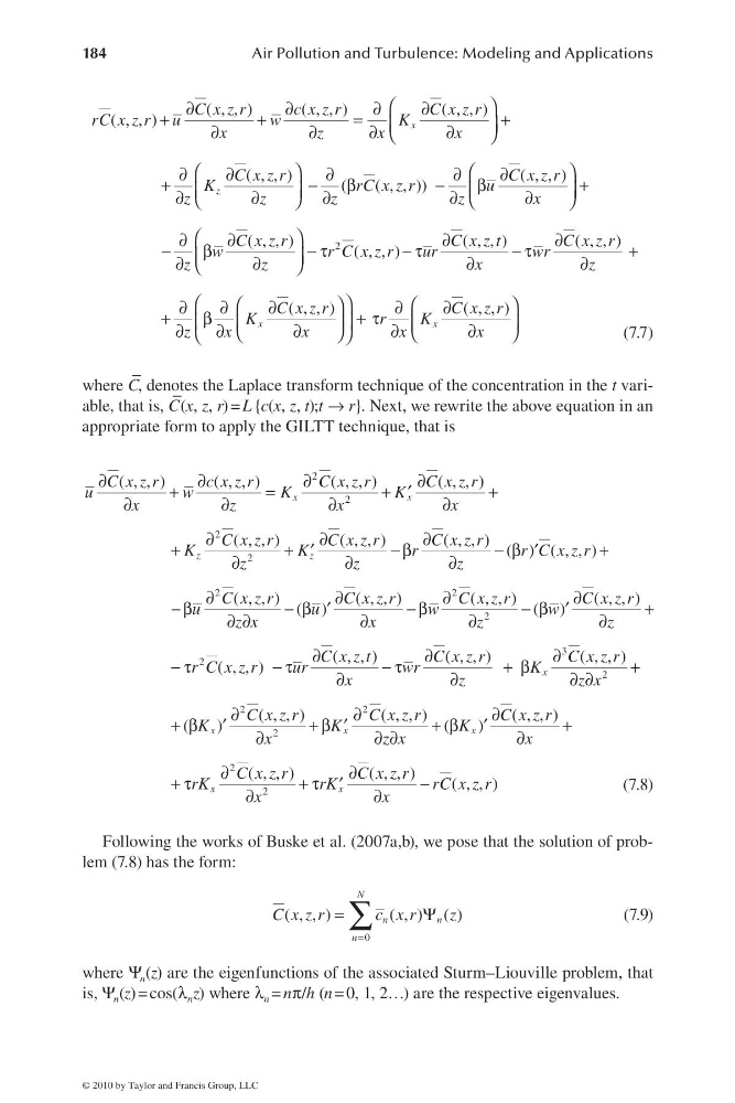
where C
–
, denotes the Laplace transform technique of the concentration in the t variable, that is, C
–
(x, z, r) = L {c(x, z, t);t → r}. Next, we rewrite the above equation in an
appropriate form to apply the GILTT technique, that is
2
2
2
2
2
2
2
2
( , , )
( , , )
( , , )
( , , )
( , , )
( , , )
( , , ) ( ) ( , , )
( , , )
( , , )
( , , )
( , , )
( )
( )
( , , )
x
x
z
z
C x z r
c x z r
C x z r
C x z r
u
w
K
K
x
z
x
x
C x z r
C x z r
C x z r
K
K
r
rCxzr
z
z
z
C x z r
C x z r
C x z r
C x z r
u
u
w
w
z x
x
z
z
r C x z r
∂
∂
∂
∂
+
=
+
+
′
∂
∂
∂
∂
∂
∂
∂
+
+
− β
−β
+
′
′
∂
∂
∂
∂
∂
∂
∂
−β
− β
−β
− β
+
′
′
∂ ∂
∂
∂
∂
− τ
− τ
3
2
2
2
2
2
2
( , , )
( , , )
( , , )
( , , )
( , , )
( , , )
(
)
(
)
( , , )
( , , )
( , , )
x
x
x
x
x
x
C x z t
C x z r
C x z r
ur
wr
K
x
z
zx
C x z r
C x z r
C x z r
K
K
K
x
zx
x
C x z r
C x z r
rK
rK
rC x z r
x
x
∂
∂
∂
− τ
+ β
+
∂
∂
∂∂
∂
∂
∂
+ β
+ β
+ β
+
′
′
′
∂
∂∂
∂
∂
∂
+ τ
+ τ
−
′
∂
∂
(7.8)
Following the works of Buske et al. (2007a,b), we pose that the solution of problem (7.8) has the form:
0
( , , )
( , ) ( )
N
n
n
n
C x z r
c x r
z
=
=
Ψ
∑
(7.9)
where Ψ n (z) are the eigenfunctions of the associated Sturm–Liouville problem, that
is, Ψ n (z) = cos(λ n z) where λ n = nπ/h (n = 0, 1, 2…) are the respective eigenvalues.
© 2010 by Taylor and Francis Group, LLC
Air Pollution and Turbulence: Modeling and Applications
2
( , , )
( , , )
( , , )
( , , )
( , , )
( , , )
(
( , , ))
( , , )
( , , )
( , , )
( , , )
x
z
x
C x z r
c x z r
C x z r
rC x z r u
w
K
x
z
x
x
C x z r
C x z r
K
r C x z r
u
z
z
z
z
x
C x z r
C x z t
C x z r
w
rCxzr
u r
w r
z
z
x
z
K
z
x
⎛
⎞
∂
∂
∂
∂
+
+
=
+
⎜
⎟
∂
∂
∂
∂
⎝
⎠
⎛
⎞
⎛
⎞
∂
∂
∂
∂
∂
+
−
β
−
β
+
⎜
⎟
⎜
⎟
∂
∂
∂
∂
∂
⎝
⎠
⎝
⎠
⎛
⎞
∂
∂
∂
∂
−
β
− τ
− τ
− τ
+
⎜
⎟
∂
∂
∂
∂
⎝
⎠
∂
∂
+
β
∂
∂
( , , )
( , , )
x
C x z r
C x z r
r
K
x
x
x
⎛
⎞
⎛
⎞
⎛
⎞
∂
∂
∂
+ τ
⎜
⎟
⎜
⎟
⎜
⎟
∂
∂
∂
⎝
⎠
⎝
⎠
⎝
⎠
(7.7)
where C
–
, denotes the Laplace transform technique of the concentration in the t variable, that is, C
–
(x, z, r) = L {c(x, z, t);t → r}. Next, we rewrite the above equation in an
appropriate form to apply the GILTT technique, that is
2
2
2
2
2
2
2
2
( , , )
( , , )
( , , )
( , , )
( , , )
( , , )
( , , ) ( ) ( , , )
( , , )
( , , )
( , , )
( , , )
( )
( )
( , , )
x
x
z
z
C x z r
c x z r
C x z r
C x z r
u
w
K
K
x
z
x
x
C x z r
C x z r
C x z r
K
K
r
rCxzr
z
z
z
C x z r
C x z r
C x z r
C x z r
u
u
w
w
z x
x
z
z
r C x z r
∂
∂
∂
∂
+
=
+
+
′
∂
∂
∂
∂
∂
∂
∂
+
+
− β
−β
+
′
′
∂
∂
∂
∂
∂
∂
∂
−β
− β
−β
− β
+
′
′
∂ ∂
∂
∂
∂
− τ
− τ
3
2
2
2
2
2
2
( , , )
( , , )
( , , )
( , , )
( , , )
( , , )
(
)
(
)
( , , )
( , , )
( , , )
x
x
x
x
x
x
C x z t
C x z r
C x z r
ur
wr
K
x
z
zx
C x z r
C x z r
C x z r
K
K
K
x
zx
x
C x z r
C x z r
rK
rK
rC x z r
x
x
∂
∂
∂
− τ
+ β
+
∂
∂
∂∂
∂
∂
∂
+ β
+ β
+ β
+
′
′
′
∂
∂∂
∂
∂
∂
+ τ
+ τ
−
′
∂
∂
(7.8)
Following the works of Buske et al. (2007a,b), we pose that the solution of problem (7.8) has the form:
0
( , , )
( , ) ( )
N
n
n
n
C x z r
c x r
z
=
=
Ψ
∑
(7.9)
where Ψ n (z) are the eigenfunctions of the associated Sturm–Liouville problem, that
is, Ψ n (z) = cos(λ n z) where λ n = nπ/h (n = 0, 1, 2…) are the respective eigenvalues.
© 2010 by Taylor and Francis Group, LLC