

168
Air Pollution and Turbulence: Modeling and Applications
physically relevant for dispersion of pollutants in the nonhomogeneous and nonstationary
atmosphere, where the varying turbulent structure of atmosphere plays a pivotal role. In
the constant K models discussed in Section 6.4.1, the solution was deduced by assuming
K’s constant and later on, their dependency on downwind distance was incorporated
through dispersion parameters at the level of application. Thus, assuming K’s constant
in derivation of the solution of advection–diffusion equation and later on introducing
their dependency on x is mathematically inconsistent (Liewelyn, 1983). However, this
approach is accepted in the applications of dispersion models. Thus, attempts have
been made to formulate variable K-models by relaxing the assumption of constant eddy
diffusivities (or dispersion parameters) in advection–diffusion equation.
6.4.2.1 Integrated Puff Model with Dispersion Parameters
as the Linear Functions of Time
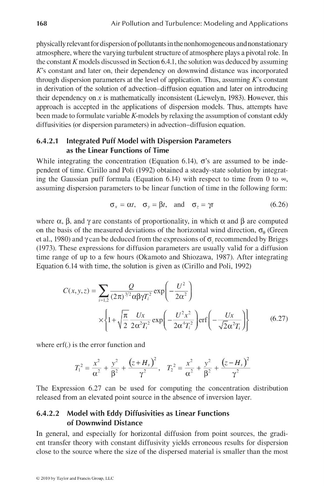
While integrating the concentration (Equation 6.14), σ’s are assumed to be independent of time. Cirillo and Poli (1992) obtained a steady-state solution by integrating the Gaussian puff formula (Equation 6.14) with respect to time from 0 to ∞,
assuming dispersion parameters to be linear function of time in the following form:
σ = α σ = β
σ = γ
,
, a n d
x
y
z
t
t
t
(6.26)
where α, β, and γ are constants of proportionality, in which α and β are computed
on the basis of the measured deviations of the horizontal wind direction, σ θ (Green
et al., 1980) and γ can be deduced from the expressions of σ z recommended by Briggs
(1973). These expressions for diffusion parameters are usually valid for a diffusion
time range of up to a few hours (Okamoto and Shiozawa, 1987). After integrating
Equation 6.14 with time, the solution is given as (Cirillo and Poli, 1992)
=
⎛
⎞
=
−
⎜
⎟
π αβγ
α
⎝
⎠
⎧
⎫
⎛
⎞
⎛
⎞
π
⎪
⎪
× +
−
−
⎨
⎬
⎜
⎟
⎜
⎟
α
α
⎝
⎠
⎝
⎠
α
⎪
⎪
⎩
⎭
∑
2
3 2
2
2
1,2
2 2
2 2
4 2
2
( , , )
exp
(2 )
2
1
exp
erf
2 2
2
2
i
i
i
i
i
Q
U
C x y z
T
Ux
U x
Ux
T
T
T
(6.27)
where erf(.) is the error function and
(
)
(
)
+
−
=
+
+
=
+
+
α
β
γ
α
β
γ
2
2
2
2
2
2
2
2
1
2
2
2
2
2
2
2
,
s
s
z H
z H
x
y
x
y
T
T
The Expression 6.27 can be used for computing the concentration distribution
released from an elevated point source in the absence of inversion layer.
6.4.2.2 Model with Eddy Diffusivities as Linear Functions
of Downwind Distance
In general, and especially for horizontal diffusion from point sources, the gradient transfer theory with constant diffusivity yields erroneous results for dispersion
close to the source where the size of the dispersed material is smaller than the most
© 2010 by Taylor and Francis Group, LLC
Air Pollution and Turbulence: Modeling and Applications
physically relevant for dispersion of pollutants in the nonhomogeneous and nonstationary
atmosphere, where the varying turbulent structure of atmosphere plays a pivotal role. In
the constant K models discussed in Section 6.4.1, the solution was deduced by assuming
K’s constant and later on, their dependency on downwind distance was incorporated
through dispersion parameters at the level of application. Thus, assuming K’s constant
in derivation of the solution of advection–diffusion equation and later on introducing
their dependency on x is mathematically inconsistent (Liewelyn, 1983). However, this
approach is accepted in the applications of dispersion models. Thus, attempts have
been made to formulate variable K-models by relaxing the assumption of constant eddy
diffusivities (or dispersion parameters) in advection–diffusion equation.
6.4.2.1 Integrated Puff Model with Dispersion Parameters
as the Linear Functions of Time
While integrating the concentration (Equation 6.14), σ’s are assumed to be independent of time. Cirillo and Poli (1992) obtained a steady-state solution by integrating the Gaussian puff formula (Equation 6.14) with respect to time from 0 to ∞,
assuming dispersion parameters to be linear function of time in the following form:
σ = α σ = β
σ = γ
,
, a n d
x
y
z
t
t
t
(6.26)
where α, β, and γ are constants of proportionality, in which α and β are computed
on the basis of the measured deviations of the horizontal wind direction, σ θ (Green
et al., 1980) and γ can be deduced from the expressions of σ z recommended by Briggs
(1973). These expressions for diffusion parameters are usually valid for a diffusion
time range of up to a few hours (Okamoto and Shiozawa, 1987). After integrating
Equation 6.14 with time, the solution is given as (Cirillo and Poli, 1992)
=
⎛
⎞
=
−
⎜
⎟
π αβγ
α
⎝
⎠
⎧
⎫
⎛
⎞
⎛
⎞
π
⎪
⎪
× +
−
−
⎨
⎬
⎜
⎟
⎜
⎟
α
α
⎝
⎠
⎝
⎠
α
⎪
⎪
⎩
⎭
∑
2
3 2
2
2
1,2
2 2
2 2
4 2
2
( , , )
exp
(2 )
2
1
exp
erf
2 2
2
2
i
i
i
i
i
Q
U
C x y z
T
Ux
U x
Ux
T
T
T
(6.27)
where erf(.) is the error function and
(
)
(
)
+
−
=
+
+
=
+
+
α
β
γ
α
β
γ
2
2
2
2
2
2
2
2
1
2
2
2
2
2
2
2
,
s
s
z H
z H
x
y
x
y
T
T
The Expression 6.27 can be used for computing the concentration distribution
released from an elevated point source in the absence of inversion layer.
6.4.2.2 Model with Eddy Diffusivities as Linear Functions
of Downwind Distance
In general, and especially for horizontal diffusion from point sources, the gradient transfer theory with constant diffusivity yields erroneous results for dispersion
close to the source where the size of the dispersed material is smaller than the most
© 2010 by Taylor and Francis Group, LLC