

160
Air Pollution and Turbulence: Modeling and Applications
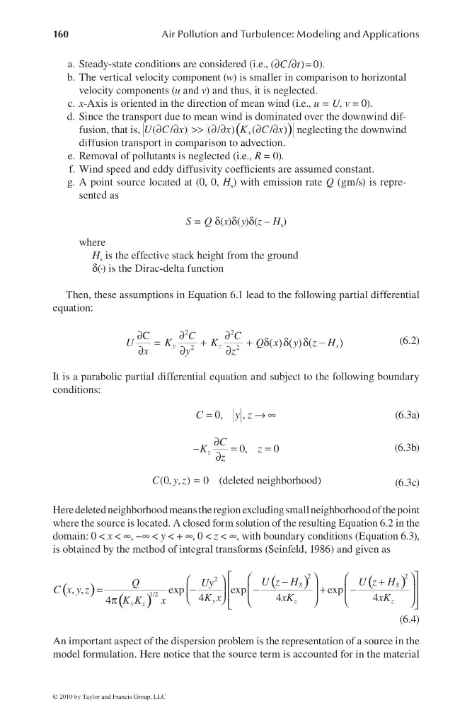
a. Steady-state conditions are considered (i.e., ∂ ∂ =
( / ) 0
C t
).
b. The vertical velocity component (w) is smaller in comparison to horizontal
velocity components (u and v) and thus, it is neglected.
c. x-Axis is oriented in the direction of mean wind (i.e., u = U, v = 0).
d. Since the transport due to mean wind is dominated over the downwind diffusion, that is,
(
)
∂ ∂ >> ∂ ∂
∂ ∂
( / )
( / )
( / )
x
U C x
x K C x neglecting the downwind
diffusion transport in comparison to advection.
e. Removal of pollutants is neglected (i.e., R = 0).
f. Wind speed and eddy diffusivity coeffi cients are assumed constant.
g. A point source located at (0, 0, H s ) with emission rate Q (gm/s) is represented as
S = Q δ(x)δ(y)δ(z – H s )
where
H s is the effective stack height from the ground
δ(·) is the Dirac-delta function
Then, these assumptions in Equation 6.1 lead to the following partial differential
equation:
∂
∂
∂
=
+
+ δ ( )δ ( )δ ( − )
∂
∂
∂
2
2
2
2
C
y
z
s
C
C
U
K
K
Q x y z H
x
y
z
(6.2)
It is a parabolic partial differential equation and subject to the following boundary
conditions:
0,
,
C
y z
=
→∞
(6.3a)
0,
0
z
C
K
z
z
∂
−
=
=
∂
(6.3b)
=
(0, , ) 0 (deleted neighborhood)
C y z
(6.3c)
Here deleted neighborhood means the region excluding small neighborhood of the point
where the source is located. A closed form solution of the resulting Equation 6.2 in the
domain: 0 < x < ∞, −∞ < y < + ∞, 0 < z < ∞, with boundary conditions (Equation 6.3),
is obtained by the method of integral transforms (Seinfeld, 1986) and given as
( )
( )
(
)
(
)
⎡
⎤
⎛
⎞
⎛
⎞
⎛
⎞
−
+
⎢
⎥
=
−
−
+
−
⎜
⎟
⎜
⎟
⎜
⎟ ⎢
⎥
⎝
⎠
π
⎝
⎠
⎝
⎠
⎣
⎦
2
2
2
1/2
, ,
exp
exp
exp
4
4
4
4
S
S
y
z
z
y z
U z H
U z H
Q
U y
C x y z
K x
xK
xK
K K
x
(6.4)
An important aspect of the dispersion problem is the representation of a source in the
model formulation. Here notice that the source term is accounted for in the material
© 2010 by Taylor and Francis Group, LLC
Air Pollution and Turbulence: Modeling and Applications
a. Steady-state conditions are considered (i.e., ∂ ∂ =
( / ) 0
C t
).
b. The vertical velocity component (w) is smaller in comparison to horizontal
velocity components (u and v) and thus, it is neglected.
c. x-Axis is oriented in the direction of mean wind (i.e., u = U, v = 0).
d. Since the transport due to mean wind is dominated over the downwind diffusion, that is,
(
)
∂ ∂ >> ∂ ∂
∂ ∂
( / )
( / )
( / )
x
U C x
x K C x neglecting the downwind
diffusion transport in comparison to advection.
e. Removal of pollutants is neglected (i.e., R = 0).
f. Wind speed and eddy diffusivity coeffi cients are assumed constant.
g. A point source located at (0, 0, H s ) with emission rate Q (gm/s) is represented as
S = Q δ(x)δ(y)δ(z – H s )
where
H s is the effective stack height from the ground
δ(·) is the Dirac-delta function
Then, these assumptions in Equation 6.1 lead to the following partial differential
equation:
∂
∂
∂
=
+
+ δ ( )δ ( )δ ( − )
∂
∂
∂
2
2
2
2
C
y
z
s
C
C
U
K
K
Q x y z H
x
y
z
(6.2)
It is a parabolic partial differential equation and subject to the following boundary
conditions:
0,
,
C
y z
=
→∞
(6.3a)
0,
0
z
C
K
z
z
∂
−
=
=
∂
(6.3b)
=
(0, , ) 0 (deleted neighborhood)
C y z
(6.3c)
Here deleted neighborhood means the region excluding small neighborhood of the point
where the source is located. A closed form solution of the resulting Equation 6.2 in the
domain: 0 < x < ∞, −∞ < y < + ∞, 0 < z < ∞, with boundary conditions (Equation 6.3),
is obtained by the method of integral transforms (Seinfeld, 1986) and given as
( )
( )
(
)
(
)
⎡
⎤
⎛
⎞
⎛
⎞
⎛
⎞
−
+
⎢
⎥
=
−
−
+
−
⎜
⎟
⎜
⎟
⎜
⎟ ⎢
⎥
⎝
⎠
π
⎝
⎠
⎝
⎠
⎣
⎦
2
2
2
1/2
, ,
exp
exp
exp
4
4
4
4
S
S
y
z
z
y z
U z H
U z H
Q
U y
C x y z
K x
xK
xK
K K
x
(6.4)
An important aspect of the dispersion problem is the representation of a source in the
model formulation. Here notice that the source term is accounted for in the material
© 2010 by Taylor and Francis Group, LLC