

158
Air Pollution and Turbulence: Modeling and Applications
compute the concentration of a contaminant at a given time and position by utilizing
available meteorological observations. An investigation of these models assists in the
planning of dispersion surveys, air quality analysis, impact assessment studies, and
emergency preparedness, and contributes to the development of strategies for future
measurement programs.
In practice, most of the estimates of dispersion are based on the Gaussian plume
model. The Gaussian model is known to work reasonably well during most of the
meteorological regimes but fails to work in weak (U < 2 m s −1 ) and variable wind
conditions (Arya, 1995; Sharan et al., 1996a,b, 2003). Pollutant dispersion in low
wind conditions becomes complicated because of the unstructured spatial and temporal behavior of the pollutants in these circumstances. The diffusion of pollutants
released from the various emission sources is irregular and indefi nite in weak and
variable wind conditions. As a consequence, no single plume centerline is obvious and the observed concentration distribution is multipeaked and non-Gaussian
(Sagendrof and Dickson, 1974). In these conditions, the state (turbulence and dispersion characteristics) of lower atmosphere is not properly understood, the pollutant
is not able to travel far, and, accordingly, the region surrounding the source may be
affected adversely. These conditions have been observed to occur for a considerable
period of time during the day as well as during the night in most parts of the world
and are sensitive due to their great potential for the occurrence of pollution episodes
(Sharan et al., 1995a, 2003; Sharan and Gopalakrishnan, 2003). For example, the
infamous Bhopal gas leak had also taken place under low wind stable conditions
(Sharan et al., 1995a).
Over the years, analytical models have been developed in the literature. These
models are essentially constrained by (1) various approximation and assumptions at
the level of formulation and (2) parameterization of dispersion parameters. During
the development of these models, a number of mathematical approximations are
involved. Some of these models have been validated using the limited available
observations. Also, some of these are successfully applied to various applications.
Thus, in this chapter, an attempt has been made to provide an overview of analytical models for the treatment of dispersion of air pollutants in low wind conditions.
6.2 GENERAL MATHEMATICAL FORMULATION
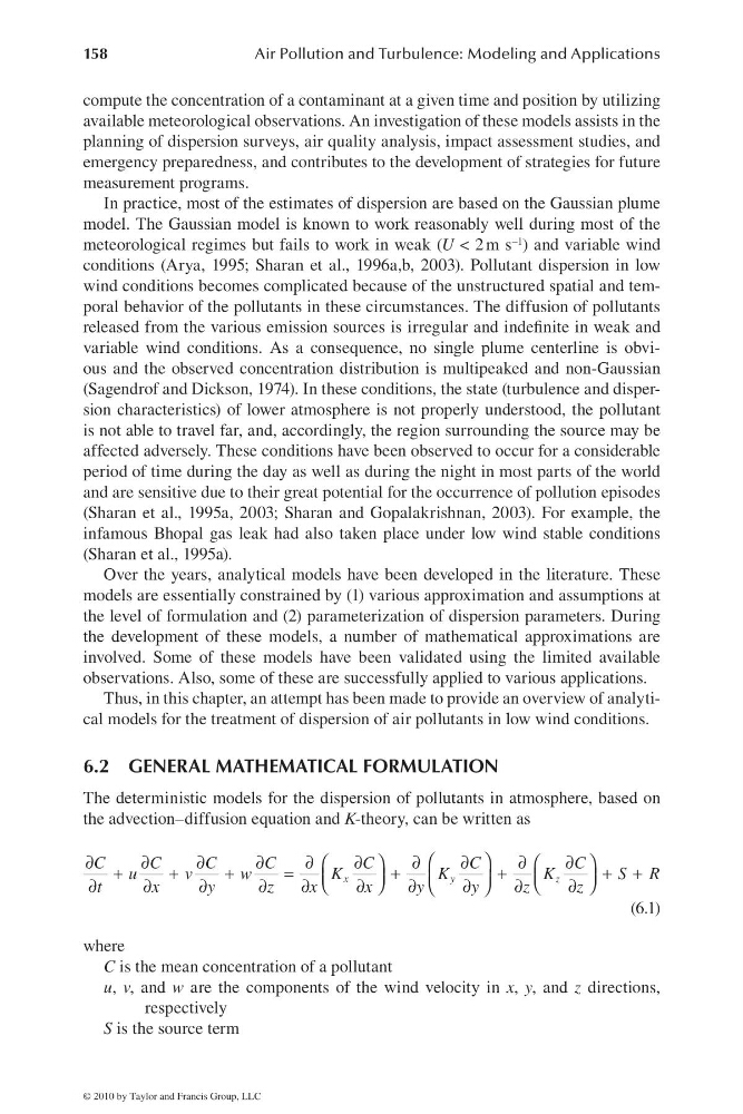
The deterministic models for the dispersion of pollutants in atmosphere, based on
the advection–diffusion equation and K-theory, can be written as
⎛
⎞
∂
∂
∂
∂
∂
∂
∂
∂
∂
∂
⎛
⎞
⎛
⎞
+
+
+
=
+
+
+ +
⎜
⎟
⎜
⎟
⎜
⎟
⎝
⎠
⎝
⎠
∂
∂
∂
∂
∂
∂
∂
∂
∂
∂
⎝
⎠
x
y
z
C
C
C
C
C
C
C
u
v
w
K
K
K
S R
t
x
y
z
x
x
y
y
z
z
(6.1)
where
C is the mean concentration of a pollutant
u, v, and w are the components of the wind velocity in x, y, and z directions,
respectively
S is the source term
© 2010 by Taylor and Francis Group, LLC
Air Pollution and Turbulence: Modeling and Applications
compute the concentration of a contaminant at a given time and position by utilizing
available meteorological observations. An investigation of these models assists in the
planning of dispersion surveys, air quality analysis, impact assessment studies, and
emergency preparedness, and contributes to the development of strategies for future
measurement programs.
In practice, most of the estimates of dispersion are based on the Gaussian plume
model. The Gaussian model is known to work reasonably well during most of the
meteorological regimes but fails to work in weak (U < 2 m s −1 ) and variable wind
conditions (Arya, 1995; Sharan et al., 1996a,b, 2003). Pollutant dispersion in low
wind conditions becomes complicated because of the unstructured spatial and temporal behavior of the pollutants in these circumstances. The diffusion of pollutants
released from the various emission sources is irregular and indefi nite in weak and
variable wind conditions. As a consequence, no single plume centerline is obvious and the observed concentration distribution is multipeaked and non-Gaussian
(Sagendrof and Dickson, 1974). In these conditions, the state (turbulence and dispersion characteristics) of lower atmosphere is not properly understood, the pollutant
is not able to travel far, and, accordingly, the region surrounding the source may be
affected adversely. These conditions have been observed to occur for a considerable
period of time during the day as well as during the night in most parts of the world
and are sensitive due to their great potential for the occurrence of pollution episodes
(Sharan et al., 1995a, 2003; Sharan and Gopalakrishnan, 2003). For example, the
infamous Bhopal gas leak had also taken place under low wind stable conditions
(Sharan et al., 1995a).
Over the years, analytical models have been developed in the literature. These
models are essentially constrained by (1) various approximation and assumptions at
the level of formulation and (2) parameterization of dispersion parameters. During
the development of these models, a number of mathematical approximations are
involved. Some of these models have been validated using the limited available
observations. Also, some of these are successfully applied to various applications.
Thus, in this chapter, an attempt has been made to provide an overview of analytical models for the treatment of dispersion of air pollutants in low wind conditions.
6.2 GENERAL MATHEMATICAL FORMULATION
The deterministic models for the dispersion of pollutants in atmosphere, based on
the advection–diffusion equation and K-theory, can be written as
⎛
⎞
∂
∂
∂
∂
∂
∂
∂
∂
∂
∂
⎛
⎞
⎛
⎞
+
+
+
=
+
+
+ +
⎜
⎟
⎜
⎟
⎜
⎟
⎝
⎠
⎝
⎠
∂
∂
∂
∂
∂
∂
∂
∂
∂
∂
⎝
⎠
x
y
z
C
C
C
C
C
C
C
u
v
w
K
K
K
S R
t
x
y
z
x
x
y
y
z
z
(6.1)
where
C is the mean concentration of a pollutant
u, v, and w are the components of the wind velocity in x, y, and z directions,
respectively
S is the source term
© 2010 by Taylor and Francis Group, LLC