

Mathematical Air Pollution Models: Eulerian Models
147
Modern expression of the “sigmas,” in terms of wind variance and the Lagrangian
integral timescale, on the basis of an atmospheric turbulence spectra model, are
presented in Mangia et al. (1998).
5.5 GAUSSIAN MODEL EXTENSIONS
As mentioned above, the Gaussian model can be modifi ed to allow the simulation of
dispersion in certain cases:
Linear, area, and volumetric sources of emission
•
Complex terrains (valleys, cities, and coastal areas)
•
Particular meteorological conditions, such as those leading to the phenom•
ena of fumigation or confi nement of pollutants
Diffusion of heavy or reactive pollutants
•
There also so-called climatological models, in which each concentration value
calculated by an equation similar to Equation 5.10 is attributed a weight, depending
on the frequency of occurrence of the meteorological conditions corresponding to
the given concentration value (Tirabassi et al., 1989; Zannetti, 1990).
To extend the range of applicability of the Gaussian method also to nonhomogeneous and nonstationary conditions, puff models have been developed. Here, the plume
emitted is subdivided into a series of independent elements, which evolve as a function
of the variation of meteorological conditions in space and time (Zanetti, 1990).
5.5.1 GAUSSIAN PUFF MODELS
Puff models were introduced to simulate the behavior of pollutants in nonhomogeneous and nonstationary meteorological and emission conditions (Zannetti, 1990).
The emission is discretized in a temporal succession of puffs, each of which shifts into
the area of calculus thanks to a three-dimensional wind fi eld that is time variable.
Gaussian puff models assume that each emission of pollutants in a time interval Δt releases into the atmosphere a mass of pollutants ΔM = QΔt, where Q is the
emission rate, which is variable in time.
Each puff contains the mass ΔM, and its baricenter is transported by the wind,
which may vary in space and time.
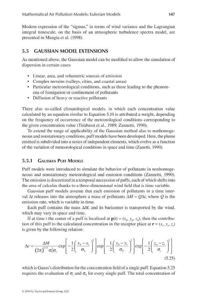
If at time t the center of a puff is localized at p(t) = (x p , y p , z p ), then the contribution of this puff to the calculated concentration in the receptor place at r = (x r , y r , z r )
is given by the following relation:
( )
2
2
2
3 / 2 2
1
1
1
exp
exp
exp
2
2
2
2
p
r
p
r
p
r
h
h
z
h z
x x
y y
z z
M
c
⎡
⎤
⎡
⎤
⎡
⎤
⎛
⎞
−
−
−
⎛
⎞
⎛
⎞
Δ
⎢
⎥
⎢
⎥
⎢
⎥
Δ =
−
−
− ⎜
⎟
⎜
⎟
⎜
⎟
σ
σ
σ
⎢
⎥
⎢
⎥
⎢
⎥
π
σ σ
⎝
⎠
⎝
⎠
⎝
⎠
⎣
⎦
⎣
⎦
⎣
⎦
(5.25)
which is Gauss’s distribution for the concentration fi eld of a single puff. Equation 5.25
requires the evaluation of σ z and σ h for every single puff. The total concentration of
© 2010 by Taylor and Francis Group, LLC
147
Modern expression of the “sigmas,” in terms of wind variance and the Lagrangian
integral timescale, on the basis of an atmospheric turbulence spectra model, are
presented in Mangia et al. (1998).
5.5 GAUSSIAN MODEL EXTENSIONS
As mentioned above, the Gaussian model can be modifi ed to allow the simulation of
dispersion in certain cases:
Linear, area, and volumetric sources of emission
•
Complex terrains (valleys, cities, and coastal areas)
•
Particular meteorological conditions, such as those leading to the phenom•
ena of fumigation or confi nement of pollutants
Diffusion of heavy or reactive pollutants
•
There also so-called climatological models, in which each concentration value
calculated by an equation similar to Equation 5.10 is attributed a weight, depending
on the frequency of occurrence of the meteorological conditions corresponding to
the given concentration value (Tirabassi et al., 1989; Zannetti, 1990).
To extend the range of applicability of the Gaussian method also to nonhomogeneous and nonstationary conditions, puff models have been developed. Here, the plume
emitted is subdivided into a series of independent elements, which evolve as a function
of the variation of meteorological conditions in space and time (Zanetti, 1990).
5.5.1 GAUSSIAN PUFF MODELS
Puff models were introduced to simulate the behavior of pollutants in nonhomogeneous and nonstationary meteorological and emission conditions (Zannetti, 1990).
The emission is discretized in a temporal succession of puffs, each of which shifts into
the area of calculus thanks to a three-dimensional wind fi eld that is time variable.
Gaussian puff models assume that each emission of pollutants in a time interval Δt releases into the atmosphere a mass of pollutants ΔM = QΔt, where Q is the
emission rate, which is variable in time.
Each puff contains the mass ΔM, and its baricenter is transported by the wind,
which may vary in space and time.
If at time t the center of a puff is localized at p(t) = (x p , y p , z p ), then the contribution of this puff to the calculated concentration in the receptor place at r = (x r , y r , z r )
is given by the following relation:
( )
2
2
2
3 / 2 2
1
1
1
exp
exp
exp
2
2
2
2
p
r
p
r
p
r
h
h
z
h z
x x
y y
z z
M
c
⎡
⎤
⎡
⎤
⎡
⎤
⎛
⎞
−
−
−
⎛
⎞
⎛
⎞
Δ
⎢
⎥
⎢
⎥
⎢
⎥
Δ =
−
−
− ⎜
⎟
⎜
⎟
⎜
⎟
σ
σ
σ
⎢
⎥
⎢
⎥
⎢
⎥
π
σ σ
⎝
⎠
⎝
⎠
⎝
⎠
⎣
⎦
⎣
⎦
⎣
⎦
(5.25)
which is Gauss’s distribution for the concentration fi eld of a single puff. Equation 5.25
requires the evaluation of σ z and σ h for every single puff. The total concentration of
© 2010 by Taylor and Francis Group, LLC