

162
10
•
Différences finies en dimension 1
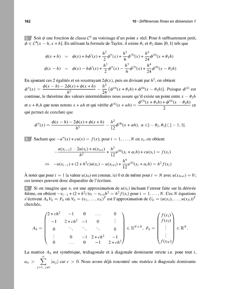
2. Soit f une fonction de classe C
4
au voisinage d’un point x réel. Pour h suffisamment petit,
f ∈C
4
[ x − h , x + h ]. En utilisant la formule de Taylor, il existe u 1 et u 2 dans ]0, 1[ tels que
f ( x + h ) = f ( x )+h f
( x )+
h
2
2
f
( x )+
h
3
6
f
(3)
( x )+
h
4
24
f
(4)
( x + u 1 h )
f ( x − h ) = f ( x ) − h f
( x )+
h
2
2
f
( x ) −
h
3
6
f
(3)
( x )+
h
4
24
f
(4)
( x − u 2 h )
En ajoutant ces 2égalités et en soustrayant 2 f ( x ), puis en divisant par h
2
,onobtient
f
( x ) =
f ( x − h ) − 2 f ( x )+f ( x + h )
h 2
−
h
2
24
f
(4)
( x + u 1 h )+f
(4)
( x − u 2 h )
.P uisque f
(4)
est
continue,lethéorème des valeurs intermédiaires nous assure qu’il existe un point entre x − u 2 h
et x + u 1 h que nous notons x + a h et qui vérifie f
(4)
( x + a h ) =
f
(4)
( x + u 1 h )+f
(4)
( x − u 2 h )
2
ce
qui permet de conclure que
f
( x ) =
f ( x − h ) − 2 f ( x )+f ( x + h )
h 2
−
h
2
12
f
(4)
( x + a h ) , a ∈ ] − u 2 , u 1 [ ⊂ ] − 1 , 1[.
3. Sachantque − u
( x )+cu( x ) = f ( x ), pour i = 1 ,...,N en x i ,onobtient
−
u ( x i − 1 ) − 2 u ( x i )+u ( x i +1 )
h 2
+
h
2
12
u
(4)
( x i + a i h )+cu( x i ) = f ( x i )
⇔− u ( x i − 1 )+(2+h
2
c ) u ( x i ) − u ( x i +1 )+
h
4
12
u
(4)
( x i + a i h ) = h
2
f ( x i )
À noter que pour i = 1lavaleur u ( x 0 )est connue, ici 0etdemême pour i = N avec u ( x N +1 ) = 0;
ces termes peuvent donc disparaître de l’écriture.
4. Si on imagine que v i est une approximation de u ( x i )i ncluant l’erreur faite sur la dérivée
4ième, on obtient − v i − 1 +(2+h
2
c ) v i − v i +1 h
2
= h
2
f ( x i )pour i = 1 ,...,N .Ces N équations
s’écrivent A h V h = F h où V h = ( v 1 ,...,v N )
T
est l’approximation de U h = ( u ( x 1 ) ,...,u ( x N ))
T
cherchée,
A h =
⎛
⎜
⎜
⎜
⎜
⎜
⎜
⎝
2+ch
2
− 10...
0
− 12 + ch
2
− 10
. . .
0
. . .
. . .
. . .
0
. . .0
− 12 + ch
2
− 1
0
...
0
− 12 + ch
2
⎞
⎟
⎟
⎟
⎟
⎟
⎟
⎠
∈ R
N × N
, F h =
⎛
⎜
⎜
⎜
⎜
⎜
⎜
⎝
f ( x 1 )
f ( x 2 )
. . .
. . .
f ( x N )
⎞
⎟
⎟
⎟
⎟
⎟
⎟
⎠
∈ R
N
.
La matrice A h est symétrique, tridiagonale et àd iagonale dominante stricte i.e. pour tout i ,
a ii >
n
j = 1 , j = i
| a ij | car c > 0. Nous avons déjà rencontré une matrice àd iagonale dominante
10
•
Différences finies en dimension 1
2. Soit f une fonction de classe C
4
au voisinage d’un point x réel. Pour h suffisamment petit,
f ∈C
4
[ x − h , x + h ]. En utilisant la formule de Taylor, il existe u 1 et u 2 dans ]0, 1[ tels que
f ( x + h ) = f ( x )+h f
( x )+
h
2
2
f
( x )+
h
3
6
f
(3)
( x )+
h
4
24
f
(4)
( x + u 1 h )
f ( x − h ) = f ( x ) − h f
( x )+
h
2
2
f
( x ) −
h
3
6
f
(3)
( x )+
h
4
24
f
(4)
( x − u 2 h )
En ajoutant ces 2égalités et en soustrayant 2 f ( x ), puis en divisant par h
2
,onobtient
f
( x ) =
f ( x − h ) − 2 f ( x )+f ( x + h )
h 2
−
h
2
24
f
(4)
( x + u 1 h )+f
(4)
( x − u 2 h )
.P uisque f
(4)
est
continue,lethéorème des valeurs intermédiaires nous assure qu’il existe un point entre x − u 2 h
et x + u 1 h que nous notons x + a h et qui vérifie f
(4)
( x + a h ) =
f
(4)
( x + u 1 h )+f
(4)
( x − u 2 h )
2
ce
qui permet de conclure que
f
( x ) =
f ( x − h ) − 2 f ( x )+f ( x + h )
h 2
−
h
2
12
f
(4)
( x + a h ) , a ∈ ] − u 2 , u 1 [ ⊂ ] − 1 , 1[.
3. Sachantque − u
( x )+cu( x ) = f ( x ), pour i = 1 ,...,N en x i ,onobtient
−
u ( x i − 1 ) − 2 u ( x i )+u ( x i +1 )
h 2
+
h
2
12
u
(4)
( x i + a i h )+cu( x i ) = f ( x i )
⇔− u ( x i − 1 )+(2+h
2
c ) u ( x i ) − u ( x i +1 )+
h
4
12
u
(4)
( x i + a i h ) = h
2
f ( x i )
À noter que pour i = 1lavaleur u ( x 0 )est connue, ici 0etdemême pour i = N avec u ( x N +1 ) = 0;
ces termes peuvent donc disparaître de l’écriture.
4. Si on imagine que v i est une approximation de u ( x i )i ncluant l’erreur faite sur la dérivée
4ième, on obtient − v i − 1 +(2+h
2
c ) v i − v i +1 h
2
= h
2
f ( x i )pour i = 1 ,...,N .Ces N équations
s’écrivent A h V h = F h où V h = ( v 1 ,...,v N )
T
est l’approximation de U h = ( u ( x 1 ) ,...,u ( x N ))
T
cherchée,
A h =
⎛
⎜
⎜
⎜
⎜
⎜
⎜
⎝
2+ch
2
− 10...
0
− 12 + ch
2
− 10
. . .
0
. . .
. . .
. . .
0
. . .0
− 12 + ch
2
− 1
0
...
0
− 12 + ch
2
⎞
⎟
⎟
⎟
⎟
⎟
⎟
⎠
∈ R
N × N
, F h =
⎛
⎜
⎜
⎜
⎜
⎜
⎜
⎝
f ( x 1 )
f ( x 2 )
. . .
. . .
f ( x N )
⎞
⎟
⎟
⎟
⎟
⎟
⎟
⎠
∈ R
N
.
La matrice A h est symétrique, tridiagonale et àd iagonale dominante stricte i.e. pour tout i ,
a ii >
n
j = 1 , j = i
| a ij | car c > 0. Nous avons déjà rencontré une matrice àd iagonale dominante