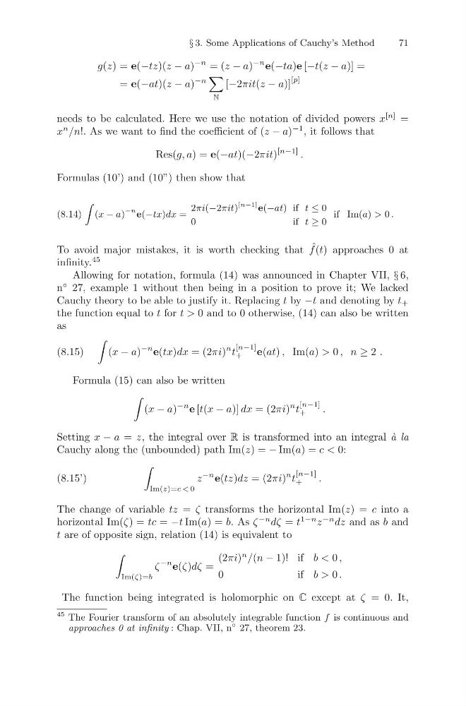
§ 3. Some Applications of Cauchy’s Method
71
g(z) = e(−tz)(z − a)
−n = (z − a)
−n e(−ta)e [−t(z − a)] =
= e(−at)(z − a)
−n
N
[−2πit(z − a)]
[p]
needs to be calculated. Here we use the notation of divided powers x
[n] =
x
n /n!. As we want to find the coefficient of (z − a)
−1 , it follows that
Res(g, a) = e(−at)(−2πit)
[n−1] .
Formulas (10’) and (10”) then show that
(x − a)
−n e(−tx)dx =
2πi(−2πit)
[n−1] e(−at) if t ≤ 0
0
i f t ≥ 0
if Im(a) > 0 .
(8.14)
To avoid major mistakes, it is worth checking that ˆ
f (t) approaches 0 at
infinity.
45
Allowing for notation, formula (14) was announced in Chapter VII, § 6,
n
◦ 27, example 1 without then being in a position to prove it; We lacked
Cauchy theory to be able to justify it. Replacing t by −t and denoting by t +
the function equal to t for t > 0 and to 0 otherwise, (14) can also be written
as
(x − a)
−n e(tx)dx = (2πi)
n t
[n−1]
+
e(at) , Im(a) > 0 , n ≥ 2 .
(8.15)
Formula (15) can also be written
(x − a)
−n e [t(x − a)] dx = (2πi)
n t
[n−1]
+
.
Setting x − a = z, the integral over R is transformed into an integral ` a la
Cauchy along the (unbounded) path Im(z) = − Im(a) = c < 0:
Im(z)=c < 0
z
−n e(tz)dz = (2πi)
n t
[n−1]
+
.
(8.15’)
The change of variable tz = ζ transforms the horizontal Im(z) = c into a
horizontal Im(ζ) = tc = −t Im(a) = b. As ζ
−n dζ = t
1−n z
−n dz and as b and
t are of opposite sign, relation (14) is equivalent to
Im(ζ)=b
ζ
−n e(ζ)dζ =
(2πi)
n /(n − 1)! if b < 0 ,
0
i f b > 0 .
The function being integrated is holomorphic on C except at ζ = 0. It,
45 The Fourier transform of an absolutely integrable function f is continuous and
approaches 0 at infinity : Chap. VII, n
◦ 27, theorem 23.