

§ 3. Integration of Differential Forms
199
Indeed the two sides are, by definition, the integrals over I
2 of the forms
( ◦ f ) ◦ σ and ◦ (σ ◦ f ). It, therefore, suffices to use (8.19) in order to
obtain (23).
(iv) A planar example. Consider the simplest case: E = R
2 . There are
two real C
1 functions f 0 and f 1 on I. Set
μ 0 (t) = (t, f 0 (t)) , μ 1 (t) = (t, f 1 (t)) ,
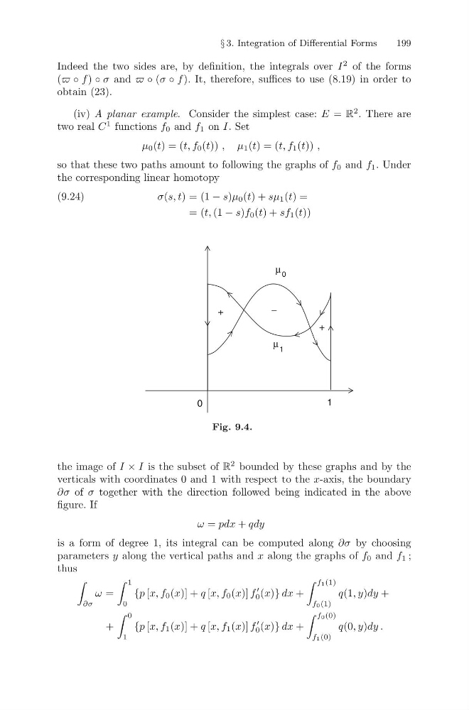
so that these two paths amount to following the graphs of f 0 and f 1 . Under
the corresponding linear homotopy
σ(s, t) = (1 − s)μ 0 (t) + sμ 1 (t) =
(9.24)
= (t, (1 − s)f 0 (t) + sf 1 (t))
+
+
−
μ
μ
0
1
1
0
Fig. 9.4.
the image of I × I is the subset of R
2 bounded by these graphs and by the
verticals with coordinates 0 and 1 with respect to the x-axis, the boundary
∂σ of σ together with the direction followed being indicated in the above
figure. If
ω = pdx + qdy
is a form of degree 1, its integral can be computed along ∂σ by choosing
parameters y along the vertical paths and x along the graphs of f 0 and f 1 ;
thus
∂σ
ω =
1
0
{p [x, f 0 (x)] + q [x, f 0 (x)] f
0 (x)} dx +
f1(1)
f0(1)
q(1, y)dy +
+
0
1
{p [x, f 1 (x)] + q [x, f 1 (x)] f
0 (x)} dx +
f0(0)
f1(0)
q(0, y)dy .
199
Indeed the two sides are, by definition, the integrals over I
2 of the forms
( ◦ f ) ◦ σ and ◦ (σ ◦ f ). It, therefore, suffices to use (8.19) in order to
obtain (23).
(iv) A planar example. Consider the simplest case: E = R
2 . There are
two real C
1 functions f 0 and f 1 on I. Set
μ 0 (t) = (t, f 0 (t)) , μ 1 (t) = (t, f 1 (t)) ,
so that these two paths amount to following the graphs of f 0 and f 1 . Under
the corresponding linear homotopy
σ(s, t) = (1 − s)μ 0 (t) + sμ 1 (t) =
(9.24)
= (t, (1 − s)f 0 (t) + sf 1 (t))
+
+
−
μ
μ
0
1
1
0
Fig. 9.4.
the image of I × I is the subset of R
2 bounded by these graphs and by the
verticals with coordinates 0 and 1 with respect to the x-axis, the boundary
∂σ of σ together with the direction followed being indicated in the above
figure. If
ω = pdx + qdy
is a form of degree 1, its integral can be computed along ∂σ by choosing
parameters y along the vertical paths and x along the graphs of f 0 and f 1 ;
thus
∂σ
ω =
1
0
{p [x, f 0 (x)] + q [x, f 0 (x)] f
0 (x)} dx +
f1(1)
f0(1)
q(1, y)dy +
+
0
1
{p [x, f 1 (x)] + q [x, f 1 (x)] f
0 (x)} dx +
f0(0)
f1(0)
q(0, y)dy .