

§ 3. Integration of Differential Forms
197
μ
ν
ν
σ
μ
1
1
0
0
σ
σ
σ
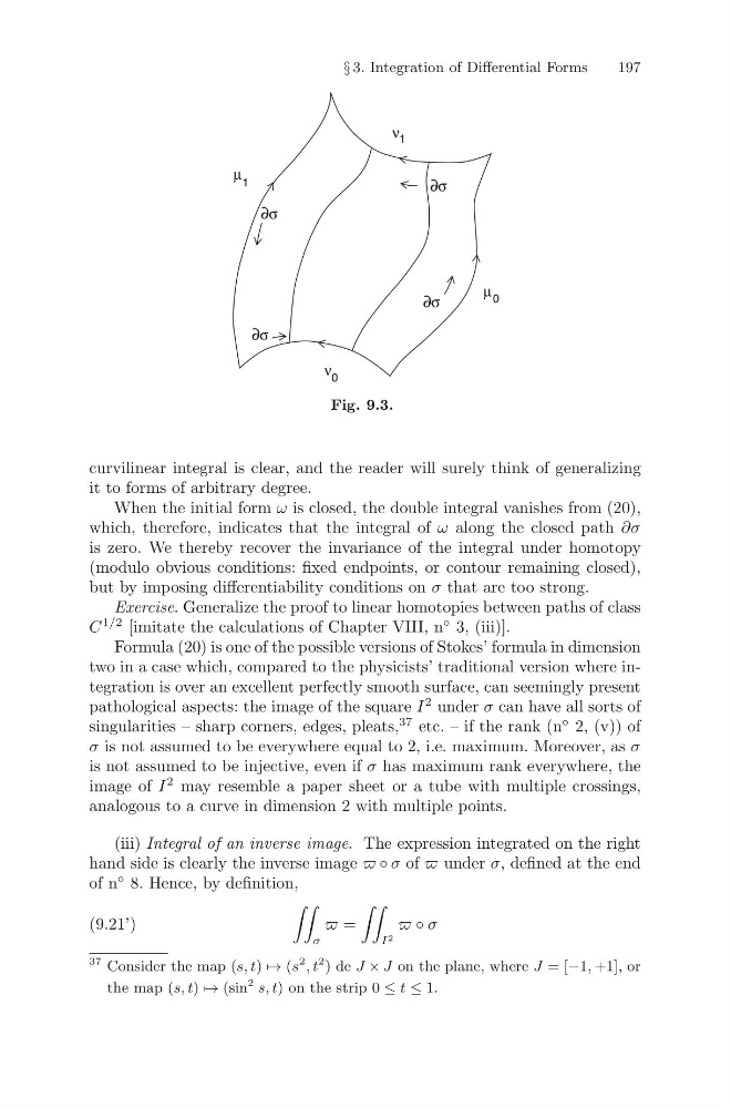
Fig. 9.3.
curvilinear integral is clear, and the reader will surely think of generalizing
it to forms of arbitrary degree.
When the initial form ω is closed, the double integral vanishes from (20),
which, therefore, indicates that the integral of ω along the closed path ∂σ
is zero. We thereby recover the invariance of the integral under homotopy
(modulo obvious conditions: fixed endpoints, or contour remaining closed),
but by imposing differentiability conditions on σ that are too strong.
Exercise. Generalize the proof to linear homotopies between paths of class
C
1/2 [imitate the calculations of Chapter VIII, n
◦ 3, (iii)].
Formula (20) is one of the possible versions of Stokes’ formula in dimension
two in a case which, compared to the physicists’ traditional version where integration is over an excellent perfectly smooth surface, can seemingly present
pathological aspects: the image of the square I
2 under σ can have all sorts of
singularities – sharp corners, edges, pleats,
37 etc. – if the rank (n
◦ 2, (v)) of
σ is not assumed to be everywhere equal to 2, i.e. maximum. Moreover, as σ
is not assumed to be injective, even if σ has maximum rank everywhere, the
image of I
2 may resemble a paper sheet or a tube with multiple crossings,
analogous to a curve in dimension 2 with multiple points.
(iii) Integral of an inverse image. The expression integrated on the right
hand side is clearly the inverse image ◦ σ of under σ, defined at the end
of n
◦ 8. Hence, by definition,
σ
=
I 2
◦ σ
(9.21’)
37 Consider the map (s, t) → (s
2 , t
2 ) de J × J on the plane, where J = [−1, +1], or
the map (s, t) → (sin
2 s, t) on the strip 0 ≤ t ≤ 1.
197
μ
ν
ν
σ
μ
1
1
0
0
σ
σ
σ
Fig. 9.3.
curvilinear integral is clear, and the reader will surely think of generalizing
it to forms of arbitrary degree.
When the initial form ω is closed, the double integral vanishes from (20),
which, therefore, indicates that the integral of ω along the closed path ∂σ
is zero. We thereby recover the invariance of the integral under homotopy
(modulo obvious conditions: fixed endpoints, or contour remaining closed),
but by imposing differentiability conditions on σ that are too strong.
Exercise. Generalize the proof to linear homotopies between paths of class
C
1/2 [imitate the calculations of Chapter VIII, n
◦ 3, (iii)].
Formula (20) is one of the possible versions of Stokes’ formula in dimension
two in a case which, compared to the physicists’ traditional version where integration is over an excellent perfectly smooth surface, can seemingly present
pathological aspects: the image of the square I
2 under σ can have all sorts of
singularities – sharp corners, edges, pleats,
37 etc. – if the rank (n
◦ 2, (v)) of
σ is not assumed to be everywhere equal to 2, i.e. maximum. Moreover, as σ
is not assumed to be injective, even if σ has maximum rank everywhere, the
image of I
2 may resemble a paper sheet or a tube with multiple crossings,
analogous to a curve in dimension 2 with multiple points.
(iii) Integral of an inverse image. The expression integrated on the right
hand side is clearly the inverse image ◦ σ of under σ, defined at the end
of n
◦ 8. Hence, by definition,
σ
=
I 2
◦ σ
(9.21’)
37 Consider the map (s, t) → (s
2 , t
2 ) de J × J on the plane, where J = [−1, +1], or
the map (s, t) → (sin
2 s, t) on the strip 0 ≤ t ≤ 1.