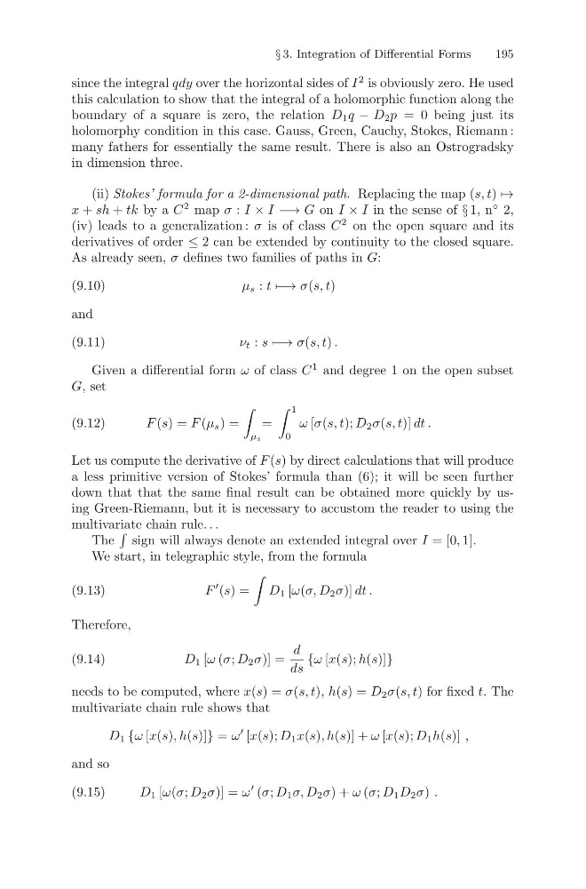
§ 3. Integration of Differential Forms
195
since the integral qdy over the horizontal sides of I
2 is obviously zero. He used
this calculation to show that the integral of a holomorphic function along the
boundary of a square is zero, the relation D 1 q − D 2 p = 0 being just its
holomorphy condition in this case. Gauss, Green, Cauchy, Stokes, Riemann :
many fathers for essentially the same result. There is also an Ostrogradsky
in dimension three.
(ii) Stokes’ formula for a 2-dimensional path. Replacing the map (s, t) →
x + sh + tk by a C
2 map σ : I × I −→ G on I × I in the sense of § 1, n
◦ 2,
(iv) leads to a generalization : σ is of class C
2 on the open square and its
derivatives of order ≤ 2 can be extended by continuity to the closed square.
As already seen, σ defines two families of paths in G:
μ s : t −→ σ(s, t)
(9.10)
and
ν t : s −→ σ(s, t) .
(9.11)
Given a differential form ω of class C
1 and degree 1 on the open subset
G, set
F (s) = F (μ s ) =
μs
=
1
0
ω [σ(s, t); D 2 σ(s, t)] dt .
(9.12)
Let us compute the derivative of F (s) by direct calculations that will produce
a less primitive version of Stokes’ formula than (6); it will be seen further
down that that the same final result can be obtained more quickly by using Green-Riemann, but it is necessary to accustom the reader to using the
multivariate chain rule. . .
The
sign will always denote an extended integral over I = [0, 1].
We start, in telegraphic style, from the formula
F
(s) =
D 1 [ω(σ, D 2 σ)] dt .
(9.13)
Therefore,
D 1 [ω (σ; D 2 σ)] =
d
ds
{ω [x(s); h(s)]}
(9.14)
needs to be computed, where x(s) = σ(s, t), h(s) = D 2 σ(s, t) for fixed t. The
multivariate chain rule shows that
D 1 {ω [x(s), h(s)]} = ω
[x(s); D 1 x(s), h(s)] + ω [x(s); D 1 h(s)] ,
and so
D 1 [ω(σ; D 2 σ)] = ω
(σ; D 1 σ, D 2 σ) + ω (σ; D 1 D 2 σ) .
(9.15)