

178
IX – Multivariate Differential and Integral Calculus
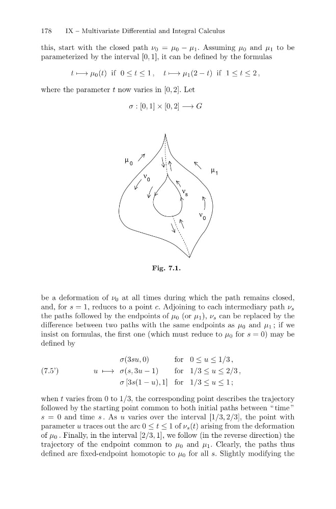
this, start with the closed path ν 0 = μ 0 − μ 1 . Assuming μ 0 and μ 1 to be
parameterized by the interval [0, 1], it can be defined by the formulas
t −→ μ 0 (t) if 0 ≤ t ≤ 1 , t −→ μ 1 (2 − t) if 1 ≤ t ≤ 2 ,
where the parameter t now varies in [0, 2]. Let
σ : [0, 1] × [0, 2] −→ G
μ
μ
ν
ν
ν
0
0
0
1
s
Fig. 7.1.
be a deformation of ν 0 at all times during which the path remains closed,
and, for s = 1, reduces to a point c. Adjoining to each intermediary path ν s
the paths followed by the endpoints of μ 0 (or μ 1 ), ν s can be replaced by the
difference between two paths with the same endpoints as μ 0 and μ 1 ; if we
insist on formulas, the first one (which must reduce to μ 0 for s = 0) may be
defined by
u −→
σ(3su, 0)
for 0 ≤ u ≤ 1/3 ,
σ(s, 3u − 1)
for 1/3 ≤ u ≤ 2/3 ,
σ [3s(1 − u), 1] for 1/3 ≤ u ≤ 1 ;
(7.5’)
when t varies from 0 to 1/3, the corresponding point describes the trajectory
followed by the starting point common to both initial paths between “ time ”
s = 0 and time s . As u varies over the interval [1/3, 2/3], the point with
parameter u traces out the arc 0 ≤ t ≤ 1 of ν s (t) arising from the deformation
of μ 0 . Finally, in the interval [2/3, 1], we follow (in the reverse direction) the
trajectory of the endpoint common to μ 0 and μ 1 . Clearly, the paths thus
defined are fixed-endpoint homotopic to μ 0 for all s. Slightly modifying the
IX – Multivariate Differential and Integral Calculus
this, start with the closed path ν 0 = μ 0 − μ 1 . Assuming μ 0 and μ 1 to be
parameterized by the interval [0, 1], it can be defined by the formulas
t −→ μ 0 (t) if 0 ≤ t ≤ 1 , t −→ μ 1 (2 − t) if 1 ≤ t ≤ 2 ,
where the parameter t now varies in [0, 2]. Let
σ : [0, 1] × [0, 2] −→ G
μ
μ
ν
ν
ν
0
0
0
1
s
Fig. 7.1.
be a deformation of ν 0 at all times during which the path remains closed,
and, for s = 1, reduces to a point c. Adjoining to each intermediary path ν s
the paths followed by the endpoints of μ 0 (or μ 1 ), ν s can be replaced by the
difference between two paths with the same endpoints as μ 0 and μ 1 ; if we
insist on formulas, the first one (which must reduce to μ 0 for s = 0) may be
defined by
u −→
σ(3su, 0)
for 0 ≤ u ≤ 1/3 ,
σ(s, 3u − 1)
for 1/3 ≤ u ≤ 2/3 ,
σ [3s(1 − u), 1] for 1/3 ≤ u ≤ 1 ;
(7.5’)
when t varies from 0 to 1/3, the corresponding point describes the trajectory
followed by the starting point common to both initial paths between “ time ”
s = 0 and time s . As u varies over the interval [1/3, 2/3], the point with
parameter u traces out the arc 0 ≤ t ≤ 1 of ν s (t) arising from the deformation
of μ 0 . Finally, in the interval [2/3, 1], we follow (in the reverse direction) the
trajectory of the endpoint common to μ 0 and μ 1 . Clearly, the paths thus
defined are fixed-endpoint homotopic to μ 0 for all s. Slightly modifying the