

§ 3. Some Applications of Cauchy’s Method
105
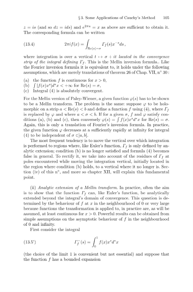
z = is (and so dz = ids) and e
2πu = x as above are sufficient to obtain it.
The corresponding formula can be written
2πif (x) =
Re(s)=σ
Γ f (s)x
−s ds ,
(13.4)
where integration is over a vertical t → σ + it located in the convergence
strip of the integral defining Γ f . This is the Mellin inversion formula.. Like
the Fourier inversion formula it is equivalent to, it holds under the following
assumptions, which are merely translations of theorem 26 of Chap. VII, n
◦ 30 :
(a) the function f is continuous for x > 0,
(b)
|f (x)x
s
|d
∗ x < +∞ for Re(s) = σ,
(c) Integral (4) is absolutely convergent.
For the Mellin version of Paley-Wiener, a given function ϕ(s) has to be shown
to be a Mellin transform. The problem is the same: suppose ϕ to be holomorphic on a strip a < Re(s) < b and define a function f using (4), where Γ f
is replaced by ϕ and where a < σ < b. If for a given σ, f and ϕ satisfy conditions (a), (b) and (c), then conversely ϕ(s) =
f (x)x
s d
∗ x for Re(s) = σ.
Again, this is only a translation of Fourier’s inversion formula. In practice,
the given function ϕ decreases at a sufficiently rapidly at infinity for integral
(4) to be independent of σ ∈]a, b[.
The most frequent tendency is to move the vertical over which integration
is performed to regions where, like Euler’s function, Γ f is only defined by analytic extension; condition (b) is no longer satisfied and formula (4) becomes
false in general. To rectify it, we take into account of the residues of Γ f at
poles encountered while moving the integration vertical, initially located in
the region where condition (b) holds, to a vertical where it no longer is. Section (iv) of this n
◦ , and more so chapter XII, will explain this fundamental
point.
(ii) Analytic extension of a Mellin transform. In practice, often the aim
is to show that the function Γ f can, like Euler’s function, be analytically
extended beyond the integral’s domain of convergence. This question is determined by the behaviour of f at x in the neighbourhood of 0 or very large
because functions the transformation is applied to, in practice are, as will be
assumed, at least continuous for x > 0. Powerful results can be obtained from
simple assumptions on the asymptotic behaviour of f in the neighbourhood
of 0 and infinity.
First consider the integral
Γ
−
f (s) =
1
0
f (x)x
s d
∗ x
(13.5’)
(the choice of the limit 1 is convenient but not essential) and suppose that
the function f has a bounded expansion
105
z = is (and so dz = ids) and e
2πu = x as above are sufficient to obtain it.
The corresponding formula can be written
2πif (x) =
Re(s)=σ
Γ f (s)x
−s ds ,
(13.4)
where integration is over a vertical t → σ + it located in the convergence
strip of the integral defining Γ f . This is the Mellin inversion formula.. Like
the Fourier inversion formula it is equivalent to, it holds under the following
assumptions, which are merely translations of theorem 26 of Chap. VII, n
◦ 30 :
(a) the function f is continuous for x > 0,
(b)
|f (x)x
s
|d
∗ x < +∞ for Re(s) = σ,
(c) Integral (4) is absolutely convergent.
For the Mellin version of Paley-Wiener, a given function ϕ(s) has to be shown
to be a Mellin transform. The problem is the same: suppose ϕ to be holomorphic on a strip a < Re(s) < b and define a function f using (4), where Γ f
is replaced by ϕ and where a < σ < b. If for a given σ, f and ϕ satisfy conditions (a), (b) and (c), then conversely ϕ(s) =
f (x)x
s d
∗ x for Re(s) = σ.
Again, this is only a translation of Fourier’s inversion formula. In practice,
the given function ϕ decreases at a sufficiently rapidly at infinity for integral
(4) to be independent of σ ∈]a, b[.
The most frequent tendency is to move the vertical over which integration
is performed to regions where, like Euler’s function, Γ f is only defined by analytic extension; condition (b) is no longer satisfied and formula (4) becomes
false in general. To rectify it, we take into account of the residues of Γ f at
poles encountered while moving the integration vertical, initially located in
the region where condition (b) holds, to a vertical where it no longer is. Section (iv) of this n
◦ , and more so chapter XII, will explain this fundamental
point.
(ii) Analytic extension of a Mellin transform. In practice, often the aim
is to show that the function Γ f can, like Euler’s function, be analytically
extended beyond the integral’s domain of convergence. This question is determined by the behaviour of f at x in the neighbourhood of 0 or very large
because functions the transformation is applied to, in practice are, as will be
assumed, at least continuous for x > 0. Powerful results can be obtained from
simple assumptions on the asymptotic behaviour of f in the neighbourhood
of 0 and infinity.
First consider the integral
Γ
−
f (s) =
1
0
f (x)x
s d
∗ x
(13.5’)
(the choice of the limit 1 is convenient but not essential) and suppose that
the function f has a bounded expansion